In the previous tutorial, I showed you how to make Handwritten sentence recognition. Now it's time for Speech recognition! Speech recognition is an essential field of Artificial Intelligence (AI) that is used to recognize a person's Speech and convert it into machine-readable text. It has many applications in many industries, such as customer service, healthcare, automotive, education, and entertainment. With the advancement in deep learning and natural language processing, speech recognition has become more accurate and efficient. This tutorial will discuss the basics of speech recognition and how to build a basic speech recognition model using TensorFlow.

History of Speech Recognition

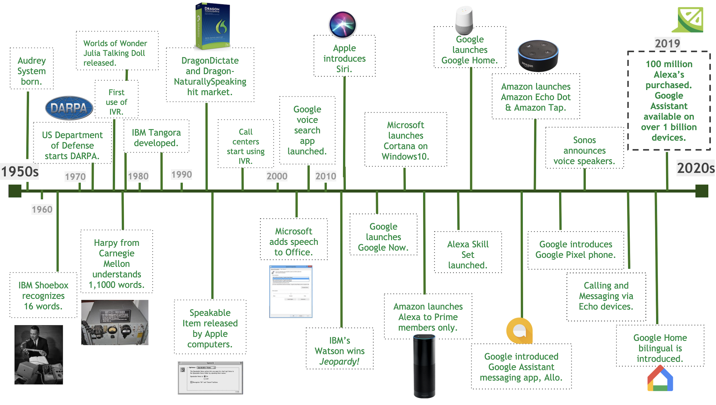
The development of speech recognition technology dates back to the 1940s when it was used for military communication and air traffic control systems. 

In the 1950s, researchers developed the first commercial speech recognition system to recognize digits spoken into a telephone. This system was limited to identifying only numbers, not full words or sentences.

In the 1960s, researchers developed more advanced speech recognition systems to recognize isolated words and short phrases. This marked a significant advancement in speech recognition, enabling machines to understand basic speech commands.

In the 1970s, researchers developed the first large-vocabulary speech recognition systems. These systems were capable of recognizing connected Speech and could handle large vocabularies. At the same time, the development of artificial neural networks and deep learning began to revolutionize the field of speech recognition. This led to the development of more accurate speech recognition systems in the 1980s. 

In the 1990s, the first commercial speech recognition products were released. These products were based on deep learning models and could be used in various applications, such as dictation software, voice-controlled user interfaces, and speech-to-text transcription services.

In the 2000s, the development of speech recognition technology continued to advance with the development of more accurate models and the incorporation of acoustic models. This led to the development of virtual assistant devices such as Google Home and Amazon Alexa.

In the 2010s, the development of deep learning algorithms further improved the accuracy of speech recognition models. In 2020, individuals utilized speech recognition technology for various purposes, ranging from customer service to healthcare and entertainment."

What are the Problems and Challenges

One of speech recognition's main challenges is dealing with human speech variability. People may have different accents, pronunciations, and speech patterns, and the model must recognize this variability accurately. Additionally, background noises and other environmental factors can interfere with the model's accuracy. 

Another challenge is dealing with words that sound similar. For example, the words "to" and "too" may sound similar but have different meanings. The model must distinguish between these words to generate an accurate output. Similarly, words with multiple meanings can be difficult for the model to interpret accurately. 

The quality of the audio signal also affects the accuracy of speech recognition. Poorly recorded audio signals can make it difficult for the model to recognize the Speech. Additionally, the model must be trained on a large dataset of audio samples to achieve a high level of accuracy. 

Finally, the model must be able to recognize and process multiple languages. Different languages have different phonetic and grammatical rules, and the model must recognize these differences to generate an accurate output. 

All of these challenges make speech recognition a difficult task. However, with the advancement of deep learning and natural language processing, speech recognition has become more accurate and efficient. With the right techniques and data, it is possible to create a high-quality speech recognition model.

Techniques in speech recognition:

The development of machine learning has significantly improved the accuracy of speech recognition. Machine learning algorithms are used to recognize complex speech patterns, understand natural language, and distinguish between different languages.

Deep learning is one of the most popular machine learning techniques in speech recognition. Deep learning uses artificial neural networks to learn from large datasets and can be used to recognize complex patterns. It has been used to develop virtual assistant devices such as Google Home and Amazon Alexa and speech-to-text transcription services.

Other machine learning techniques used in speech recognition include Hidden Markov Models (HMM), Dynamic Time Warping (DTW), and phonetic-based approaches. HMM is a statistical approach for modeling time series data and is used for recognizing speech patterns. DTW is a technique used for comparing two temporal sequences and is used for recognizing similar speech patterns. Phonetic-based approaches recognize Speech based on their phonetic similarity.

Additionally, there are techniques for improving the accuracy of speech recognition models. Beamforming is a technique that reduces background noise by focusing on the sound source. Noise cancellation is a technique used to reduce background noise by subtracting it from the audio signal. Both of these techniques can improve the accuracy of speech recognition models.

Until 2018, the most common technique in Speech Recognition was Deep Neural Networks with LSTM, and everything changed when transformers were released. When Transformers were released, they significantly impacted the field of speech recognition. The Transformers are a type of neural network used for natural language processing tasks and to recognize complex patterns in the input audio. They are beneficial for tasks such as speech recognition because they can model long-term dependencies in the data. 

The introduction of Transformers has allowed for more accurate speech recognition models. You can use them to recognize different languages, understand natural language, and distinguish between similar words. The increased accuracy of these models has enabled the development of virtual assistant devices, voice-controlled user interfaces, and speech-to-text transcription services.

Implementation:

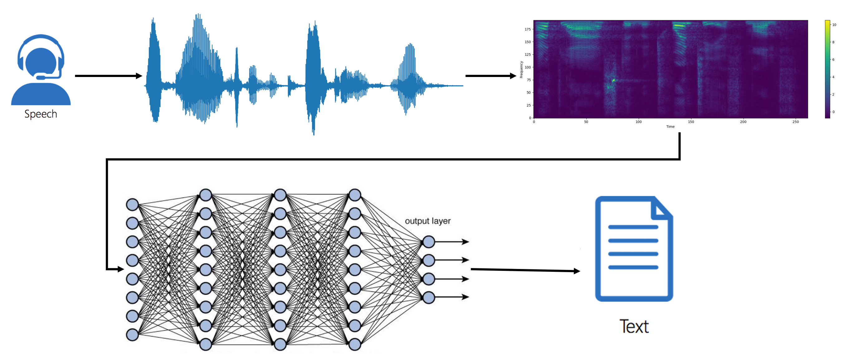
In this tutorial, I will demonstrate how to combine a 2D convolutional neural network (CNN), recurrent neural network (RNN), and a Connectionist Temporal Classification (CTC) loss to build an automatic speech recognition (ASR) model. 

This tutorial will utilize the LJSpeech dataset, which features brief audio recordings of a solitary speaker reciting passages from seven non-fiction books. 

To gauge the effectiveness of our model, we'll employ the Word Error Rate (WER) and Character Error Rate (CER) evaluation metrics. These metrics calculate the discrepancy between the recognized words/characters and the original spoken words/characters. WER is determined by summing up the number of substitutions, insertions, and deletions that occur in the sequence of recognized words and dividing the result by the total number of initially spoken words. CER follows the same principle but on a character level.

Prerequisites:

Before we begin, you will need to have the following software installed:

• Python 3;
• TensorFlow (We will be using version 2.10 in this tutorial);
• mltu==0.1.7

The LJSpeech Dataset:

We'll begin by downloading the LJSpeech Dataset. This dataset contains 13000 audio files in a ".wav" format. All the actual labels are also given to us in the annotation file.

To simplify this for us a little, I wrote a short script that we'll use to download this dataset:

import stow
import tarfile
import pandas as pd
from tqdm import tqdm
from urllib.request import urlopen
from io import BytesIO

def download_and_unzip(url, extract_to='Datasets', chunk_size=1024*1024):
    http_response = urlopen(url)

    data = b''
    iterations = http_response.length // chunk_size + 1
    for _ in tqdm(range(iterations)):
        data += http_response.read(chunk_size)

    tarFile = tarfile.open(fileobj=BytesIO(data), mode='r|bz2')
    tarFile.extractall(path=extract_to)
    tarFile.close()

dataset_path = stow.join('Datasets', 'LJSpeech-1.1')
if not stow.exists(dataset_path):
    download_and_unzip('https://data.keithito.com/data/speech/LJSpeech-1.1.tar.bz2', extract_to='Datasets')

Likely a slower method to download this dataset, but you don't need to do anything manually. 

Now we have our dataset downloaded, and we need to preprocess it before moving forward to another step. Preprocessing consists of several steps. All the preprocessing we can do with the following code:

dataset_path = "Datasets/LJSpeech-1.1"
metadata_path = dataset_path + "/metadata.csv"
wavs_path = dataset_path + "/wavs/"

# Read metadata file and parse it
metadata_df = pd.read_csv(metadata_path, sep="|", header=None, quoting=3)
metadata_df.columns = ["file_name", "transcription", "normalized_transcription"]
metadata_df = metadata_df[["file_name", "normalized_transcription"]]

# structure the dataset where each row is a list of [wav_file_path, sound transcription]
dataset = [[f"Datasets/LJSpeech-1.1/wavs/{file}.wav", label] for file, label in metadata_df.values.tolist()]

# Create a ModelConfigs object to store model configurations
configs = ModelConfigs()

max_text_length, max_spectrogram_length = 0, 0
for file_path, label in tqdm(dataset):
    spectrogram = WavReader.get_spectrogram(file_path, frame_length=configs.frame_length, frame_step=configs.frame_step, fft_length=configs.fft_length)
    valid_label = [c for c in label.lower() if c in configs.vocab]
    max_text_length = max(max_text_length, len(valid_label))
    max_spectrogram_length = max(max_spectrogram_length, spectrogram.shape[0])
    configs.input_shape = [max_spectrogram_length, spectrogram.shape[1]]

configs.max_spectrogram_length = max_spectrogram_length
configs.max_text_length = max_text_length
configs.save()

First, we are loading raw audio data with librosa.load(audio_path) from the Python library librosa. It loads an audio file specified by the audio_path parameter and returns a tuple of two objects: The raw audio signal as a NumPy array, representing the audio samples and the sample rate (number of samples per second) of the audio signal, typically defined as an integer. So, we are iterating through dataset metadata and preprocessing the 'wav' audio data with actual transcription. It looks as follows:

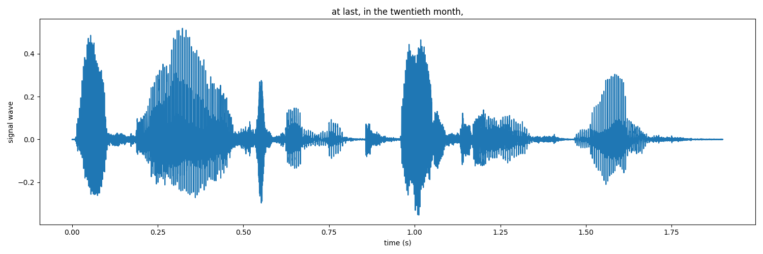
Then we preprocess this rad audio data further to receive a spectrogram that we will use to train our model. 

An audio spectrogram is a visual representation of the frequency content of an audio signal over time. It displays the signal's power spectral density (PSD), which gives a measure of the strength of different frequency components of the signal.

The spectrogram is usually represented as an image. The X-axis represents time, the Y-axis represents frequency, and the color or brightness represents the magnitude of the frequency components at each time frame. The brighter the color or higher the brightness, the higher the magnitude of the corresponding frequency component.

Spectrograms are commonly used in audio analysis and processing, as they provide a clear representation of the frequency content of a signal and can reveal important information such as pitch, harmonics, and transient events. They are also useful for identifying different types of sounds and for performing tasks such as noise reduction, pitch correction, and audio compression.

An example of an audio spectrogram would look following:

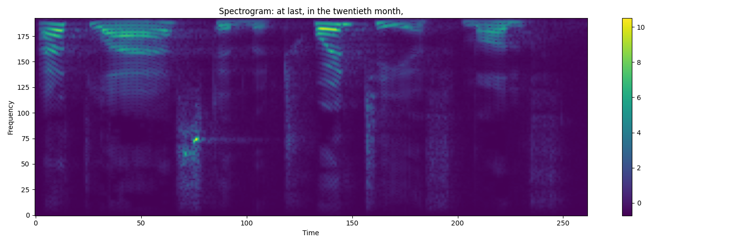
Keep in mind that when we were iterating through actual transcription, we replaced all capital letters with lower ones and removed all unusual alphabet letters.

When we prepare our dataset, we can create our TensorFlow data provider, which will provide us with data through all the training processes; we won't need to hold all the data on RAM. 

As before, I will use my "mltu" package:

# Create a data provider for the dataset
data_provider = DataProvider(
    dataset=dataset,
    skip_validation=True,
    batch_size=configs.batch_size,
    data_preprocessors=[
        WavReader(frame_length=configs.frame_length, frame_step=configs.frame_step, fft_length=configs.fft_length),
        ],
    transformers=[
        SpectrogramPadding(max_spectrogram_length=configs.max_spectrogram_length, padding_value=0),
        LabelIndexer(configs.vocab),
        LabelPadding(max_word_length=configs.max_text_length, padding_value=len(configs.vocab)),
        ],
)

You may notice that I am using the WavReader as the data preprocessor and SpectrogramPadding, LabelIndexer, and LabelPadding as transformers. In the given code, the purpose of each component is as follows:

1. WavReader: This class reads audio files (in WAV format) and converts them into spectrograms. It uses the parameters frame_length, frame_step, and fft_length to determine how the audio signals should be split into frames and transformed into spectrograms.
2. SpectrogramPadding: This class is used to pad spectrograms to a consistent length so that all spectrograms in a batch have the same shape. It uses the parameter max_spectrogram_length to determine the length to which the spectrograms should be padded and the padding_value to determine the value used for padding.
3. LabelIndexer: This class converts text labels into numerical representations, for example, transforming words into integers. It uses the vocab parameter, a dictionary of all the words in the vocabulary, to determine how to map words to integers.
4. LabelPadding: This class is used to pad text labels to a consistent length so that all text labels in a batch have the same length. It uses the parameter max_word_length to determine the length to which the text labels should be padded and the padding_value to determine the value used for padding.

These components are used together to preprocess the data before it is fed into a machine-learning model. By preprocessing the data this way, it becomes easier to train a model on the data and ensure that the model receives a consistent input format.

When training the model, we can't rely on training loss. For this purpose, we'll split the dataset into the training 90% and validation 10%:

# Split the dataset into training and validation sets
train_data_provider, val_data_provider = data_provider.split(split = 0.9)

The model architecture:

CNNs for speech recognition: Convolutional Neural Networks are a type of machine learning architecture that is mostly used for analyzing visual datasets. They are good at analyzing images because they can pick up on the spatial and temporal relationships between the pixels in the image. 

The convolution layer examines the essential features of the input data, and the subsampling layer compresses these features into a more straightforward form.

For speech recognition, CNNs take a spectrogram of the speech signal, which is represented as an image, and use these features to recognize speech.

RNNs for speech recognition: Recurrent Neural Networks are a type of deep learning architecture that can handle large sequential inputs. The key idea behind RNNs is that they use the current information and previous inputs to produce the current output. This makes them well-suited for sequential data tasks, such as natural language processing and speech recognition.

RNNs are the preferred deep learning architecture for speech recognition because they are good at modeling sequential data. They can capture the long-term dependencies between the features in the input dataset and produce outputs based on past observations. This is particularly useful for speech recognition tasks because the output of a speech frame depends on previous frames of observations. RNNs and their improved version, Long-Short Term Memory (LSTM) RNNs, have the best performance (Except Transformers) for speech recognition tasks among all deep learning architectures and are the preferred choice.

So we'll define our model:

# Creating TensorFlow model architecture
model = train_model(
    input_dim = configs.input_shape,
    output_dim = len(configs.vocab),
    dropout=0.5
)

For a deeper understanding of the architecture, we can open our model.py file, where we create the TensorFlow sequential model step-by-step:

import tensorflow as tf
from keras import layers
from keras.models import Model

from mltu.model_utils import residual_block, activation_layer

def train_model(input_dim, output_dim, activation='leaky_relu', dropout=0.2):
    
    inputs = layers.Input(shape=input_dim, name="input")

    # expand dims to add channel dimension
    input = layers.Lambda(lambda x: tf.expand_dims(x, axis=-1))(inputs)

    # Convolution layer 1
    x = layers.Conv2D(filters=32, kernel_size=[11, 41], strides=[2, 2], padding="same", use_bias=False)(input)
    x = layers.BatchNormalization()(x)
    x = activation_layer(x, activation='leaky_relu')

    # Convolution layer 2
    x = layers.Conv2D(filters=32, kernel_size=[11, 21], strides=[1, 2], padding="same", use_bias=False)(x)
    x = layers.BatchNormalization()(x)
    x = activation_layer(x, activation='leaky_relu')
    
    # Reshape the resulted volume to feed the RNNs layers
    x = layers.Reshape((-1, x.shape[-2] * x.shape[-1]))(x)

    # RNN layers
    x = layers.Bidirectional(layers.LSTM(128, return_sequences=True))(x)
    x = layers.Dropout(dropout)(x)

    x = layers.Bidirectional(layers.LSTM(128, return_sequences=True))(x)
    x = layers.Dropout(dropout)(x)

    x = layers.Bidirectional(layers.LSTM(128, return_sequences=True))(x)
    x = layers.Dropout(dropout)(x)

    x = layers.Bidirectional(layers.LSTM(128, return_sequences=True))(x)
    x = layers.Dropout(dropout)(x)

    x = layers.Bidirectional(layers.LSTM(128, return_sequences=True))(x)

    # Dense layer
    x = layers.Dense(256)(x)
    x = activation_layer(x, activation='leaky_relu')
    x = layers.Dropout(dropout)(x)

    # Classification layer
    output = layers.Dense(output_dim + 1, activation="softmax")(x)
    
    model = Model(inputs=inputs, outputs=output)
    return model

Great, now we have the model that we need to compile. Let's do it:

# Compile the model
model.compile(
    optimizer=tf.keras.optimizers.Adam(learning_rate=configs.learning_rate), 
    loss=CTCloss(), 
    metrics=[
        CERMetric(vocabulary=configs.vocab),
        WERMetric(vocabulary=configs.vocab)
        ],
    run_eagerly=False
)

As you might notice, I am using CTCloss and custom CER and WER metrics. CER and WER I introduced in my previous tutorials, but these also are one of the most common metrics to tell how accurate our predictions are from actual transcription. CTC is the most common loss when training stuff related to language recognition and extraction.

Now, we can define our callbacks (introduced in previous tutorials) and start the training process:

# Define callbacks
earlystopper = EarlyStopping(monitor='val_CER', patience=20, verbose=1, mode='min')
checkpoint = ModelCheckpoint(f"{configs.model_path}/model.h5", monitor='val_CER', verbose=1, save_best_only=True, mode='min')
trainLogger = TrainLogger(configs.model_path)
tb_callback = TensorBoard(f'{configs.model_path}/logs', update_freq=1)
reduceLROnPlat = ReduceLROnPlateau(monitor='val_CER', factor=0.8, min_delta=1e-10, patience=5, verbose=1, mode='auto')
model2onnx = Model2onnx(f"{configs.model_path}/model.h5")

# Train the model
model.fit(
    train_data_provider,
    validation_data=val_data_provider,
    epochs=configs.train_epochs,
    callbacks=[earlystopper, checkpoint, trainLogger, reduceLROnPlat, tb_callback, model2onnx],
    workers=configs.train_workers
)

# Save training and validation datasets as csv files
train_data_provider.to_csv(stow.join(configs.model_path, 'train.csv'))
val_data_provider.to_csv(stow.join(configs.model_path, 'val.csv'))

Training process:

To track the training process, we added the TensorBoard metric, there we can check what our curves of loss, CER, and WER metrics were. Here is the loss curve:

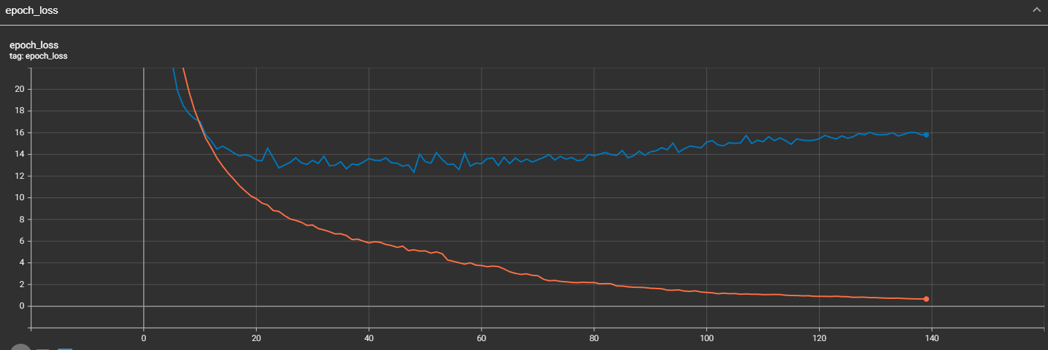
We can see that while training, our loss was constantly decreasing; that's what we expected to see. But we might see that validation loss was falling since the 48 training step, and then it increased. This means our mode might be overfitting. We may see similar scenarios in our CER and WER curves. Let's take a look at them. Here is the CER curve:

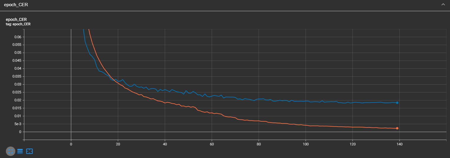
I was wrong; the CER of validation was constantly improving until step 100. But we can see here a huge gap between training and validation CERs. This is because we are not using any augmentation techniques for our audio data. Let's look at the WER curve:

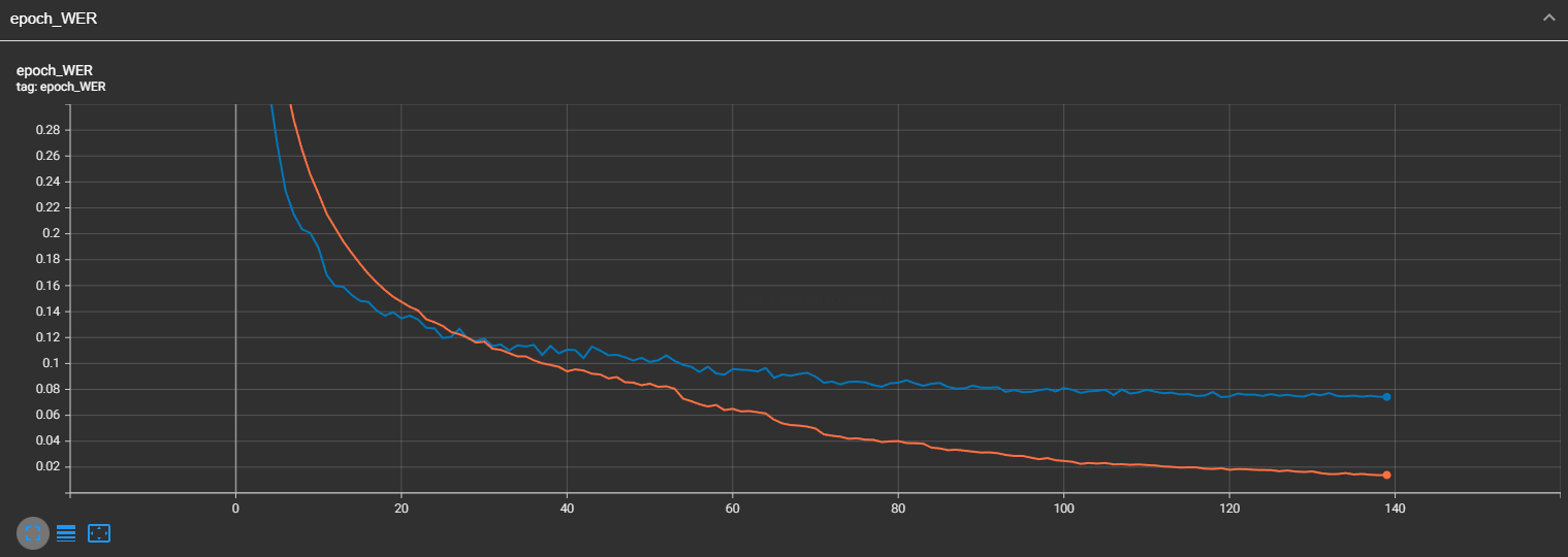
It looks very similar to CER; that's what I was expecting. But overall, our CER is only 1.7%, and our WER is 7%. This means that our model performs well on this dataset!

Test model inference:

Our model is trained, and it gave us pretty satisfying results. How can we test it out on single inference? I wrote a script that iterates through validation data from our training data:

import typing
import numpy as np

from mltu.inferenceModel import OnnxInferenceModel
from mltu.preprocessors import WavReader
from mltu.utils.text_utils import ctc_decoder, get_cer, get_wer

class WavToTextModel(OnnxInferenceModel):
    def __init__(self, char_list: typing.Union[str, list], *args, **kwargs):
        super().__init__(*args, **kwargs)
        self.char_list = char_list

    def predict(self, data: np.ndarray):
        data_pred = np.expand_dims(data, axis=0)

        preds = self.model.run(None, {self.input_name: data_pred})[0]

        text = ctc_decoder(preds, self.char_list)[0]

        return text

if __name__ == "__main__":
    import pandas as pd
    from tqdm import tqdm
    from mltu.configs import BaseModelConfigs

    configs = BaseModelConfigs.load("Models/05_sound_to_text/202302051936/configs.yaml")

    model = WavToTextModel(model_path=configs.model_path, char_list=configs.vocab, force_cpu=False)

    df = pd.read_csv("Models/05_sound_to_text/202302051936/val.csv").values.tolist()

    accum_cer, accum_wer = [], []
    for wav_path, label in tqdm(df):
        
        spectrogram = WavReader.get_spectrogram(wav_path, frame_length=configs.frame_length, frame_step=configs.frame_step, fft_length=configs.fft_length)
        # WavReader.plot_raw_audio(wav_path, label)

        padded_spectrogram = np.pad(spectrogram, (0, (configs.max_spectrogram_length - spectrogram.shape[0]),(0,0)), mode='constant', constant_values=0)

        # WavReader.plot_spectrogram(spectrogram, label)

        text = model.predict(padded_spectrogram)

        true_label = "".join([l for l in label.lower() if l in configs.vocab])

        cer = get_cer(text, true_label)
        wer = get_wer(text, true_label)

        accum_cer.append(cer)
        accum_wer.append(wer)

    print(f"Average CER: {np.average(accum_cer)}, Average WER: {np.average(accum_wer)}")

If you want to test this on your recording, remove the iterative loop and link our audio 'wav' recording, it should handle it! The trained model can be downloaded from this link. 

Conclusion:

Speech recognition is a field of AI with a rich history of advancements dating back to the 1940s. With deep learning and natural language processing integration, speech recognition has become more accurate and efficient. The main challenges in speech recognition include the following:

• Dealing with human speech variability;
• Recognizing similar words;
• The quality of the audio signal.

Several techniques are used in speech recognition, including Deep learning, Hidden Markov Models, Dynamic Time Warping, and phonetic-based approaches. Additionally, beamforming and noise cancellation techniques can be used to improve the accuracy of speech recognition models. 

The introduction of transformers has significantly impacted speech recognition, enabling more accurate models for tasks such as speech recognition, natural language processing, and virtual assistant devices. 

This tutorial demonstrated how to build a basic speech recognition model using TensorFlow by combining a 2D CNN, RNN, and CTC loss. With the right techniques and data, speech recognition can be a powerful tool for many industries.

The trained model used in this tutorial can be downloaded from this link.

Complete tutorial code on GitHub.