In the previous post, we covered simple DCGAN, and I gave you a simple example with the MNIST dataset. But it was a simple dataset, and we could not see the disadvantages of this architecture. The main disadvantage is its training instability; over time, it gives us worse and worse generated images.
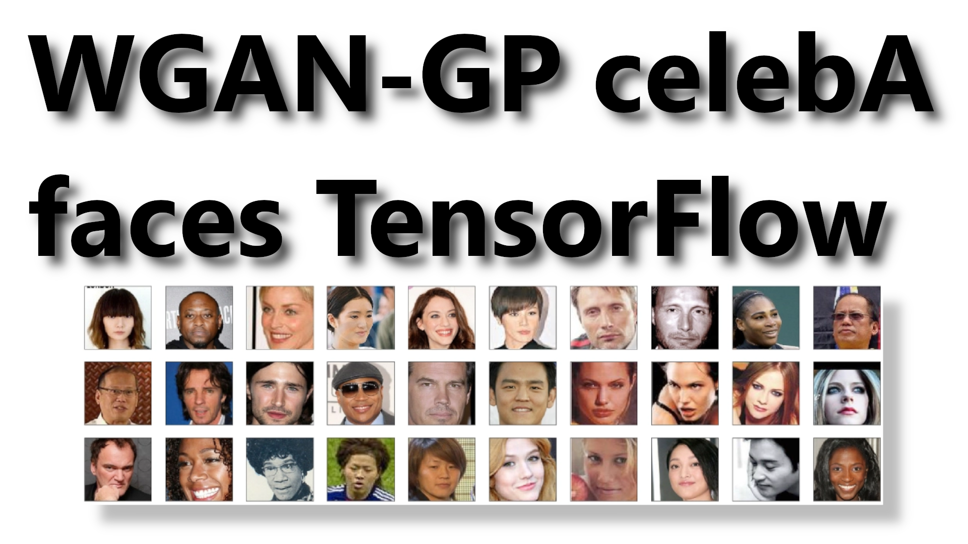
So, to address this issue, we will implement a WGAN-GP (Wasserstein GAN with Gradient Penalty) architecture. We will train the WGAN-GP model to generate people's profile 64x64 images by training it on the popular CelebA dataset.
Wasserstein GAN
The Wasserstein GAN, or WGAN, was a breakthrough in Generative Adversarial Network (GAN) training when it was introduced in the paper of the same name. Using the Wasserstein loss, it addressed the instability issues that had plagued traditional GAN training.
One of the main issues with Deep Convolutional GANs (DCGANs) is that when the discriminator is too weak or too strong, it doesn't provide the generator with useful feedback for improvement. This makes it challenging to improve the DCGAN model even with extended training.
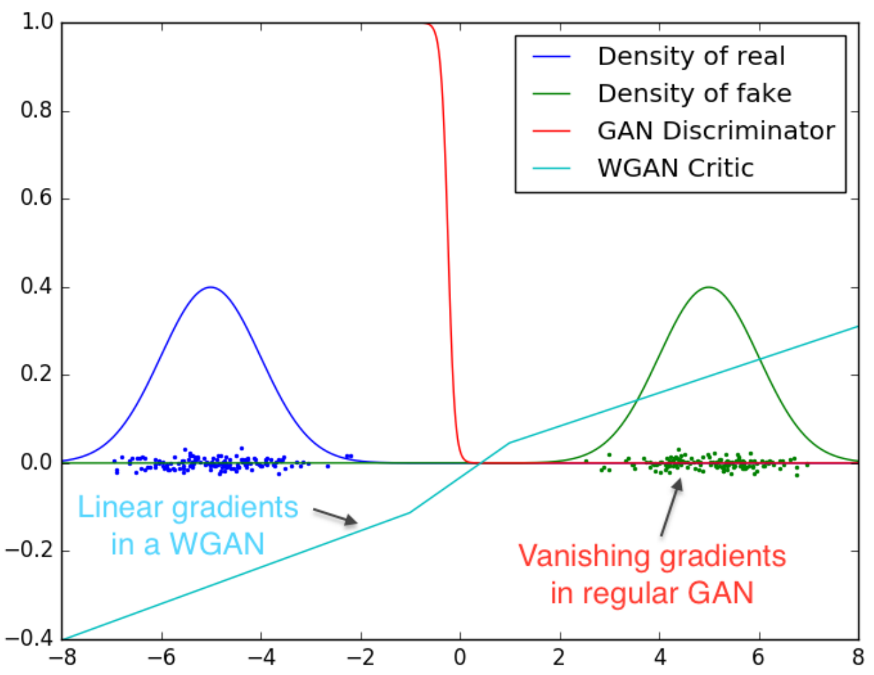
However, WGAN overcomes these issues by using the Wasserstein loss. This new method eliminated the need for carefully balanced training of the discriminator and generator or meticulous network architecture design. Additionally, WGAN has continuous and differentiable linear gradients that solve the vanishing gradient problem in traditional GAN training.
Wasserstein GAN with Gradient Penalty
Although the Wasserstein GAN (WGAN) uses the Wasserstein loss to improve training stability, it has a significant issue with enforcing the 1-Lipschitz constraint. In fact, the authors of WGAN acknowledged in their paper that "weight clipping is a clearly terrible way" to impose this constraint. If the clipping parameter is set to a large value, it can slow down the training process and also hinder the critic from achieving optimal performance. In contrast, a small clipping parameter can cause vanishing gradients, which defeats the purpose of using WGAN in the first place.
The issue mentioned above was tackled by introducing a new technique called Wasserstein with Gradient Penalty (WGAN-GP) in the research paper "improved Training of Wasserstein GANs.". WGAN-GP differs from WGAN in that it enforces the 1-Lipschitz constraint for the critic by adding a gradient penalty instead of relying on weight clipping. This improvement helps avoid weight clipping issues and provides more stable training for GANs.
So, I don't see a reason to focus on a simple WGAN architecture because WGAN-GP solved its issues.
I strongly recommend getting familiar with my previous tutorial, where I walked through DCGAN architecture and implementation in TensorFlow. In this part, I'll continue and go step-by-step about what changes we need to make to convert our DCGAN architecture into WGAN-GP!
Prerequisites:
For this tutorial, we'll use Python 3.10 and TensorFlow 2.10, so make sure you have them. Other required packages may be found in the requirements.txt file. Make sure you have them also. All project files can be found on GitHub.
Prepare the Data
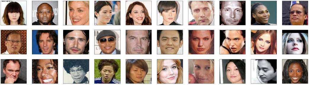
We will train the WGAN-GP with a CelebFaces Attributes Dataset (CelebA). It is a large-scale face attributes dataset with over 200K celebrity images.
You can download this Dataset from Kaggle. Extract the "img_align_celeba" folder into the Datasets repository.
This tutorial will resize all images to 64x64 pixel size as discriminator input. For Discriminator, we'll use a noise dimension of 128. So we'll use the following preprocessing code:
# celebA dataset path
dataset_path = "Dataset/img_align_celeba"

# Set the input shape and size for the generator and discriminator
batch_size = 128
img_shape = (64, 64, 3) # The shape of the input image, input to the discriminator
noise_dim = 128 # The dimension of the noise vector, input to the generator
model_path = 'Models/02_WGANGP_faces'
os.makedirs(model_path, exist_ok=True)

# Define your data generator
datagen = ImageDataGenerator(
    preprocessing_function=lambda x: (x / 127.5) - 1.0,  # Normalize image pixel values to [-1, 1]
    horizontal_flip=True  # Data augmentation
)

# Create a generator that yields batches of images
train_generator = datagen.flow_from_directory(
    directory=dataset_path,  # Path to directory containing images
    target_size=img_shape[:2],  # Size of images (height, width)
    batch_size=batch_size,
    class_mode=None,  # Do not use labels
    shuffle=True,  # Shuffle the data
)
Here, we set the path where we put CelebA dataset files, we set image input and noise dimensions, and we set the path for models.
Next, we could load all images from the given path, resize them to our specified image size, and place them into the list. But this would use around 24 GB of RAM; we don't want this. To overcome this issue, we are creating ImageDataGenerator, where we normalize the images to the [-1, 1] range because the generator's final layer activation uses "tanh". Although, we use one augmentation technique - "horizontal flip".
Next, we define a train_generator with our dataset path, image shape, batch size, etc.
Here are a few examples from the CelebA dataset:
The Generator
There is no change in the WGAN-GP Generator architecture, which is the same as in DCGAN (from the previous tutorial). Compared to the last implementation tutorial, we are using the same logic. Still, we are increasing the filters count in Conv2D layers because generating people's faces is more challenging than simple DIGITS. Here is the generator model:
import tensorflow as tf
from keras import layers

# Define the generator model
def build_generator(noise_dim, output_channels=3, activation="tanh", alpha=0.2):
    inputs = layers.Input(shape=noise_dim, name="input")

    x = layers.Dense(4*4*512, use_bias=False)(inputs)

    x = layers.Reshape((4, 4, 512))(x)

    x = layers.Conv2DTranspose(512, (5, 5), strides=(2, 2), padding="same", use_bias=False)(x)
    x = layers.BatchNormalization()(x)
    x = layers.LeakyReLU(alpha)(x)

    x = layers.Conv2DTranspose(256, (5, 5), strides=(2, 2), padding="same", use_bias=False)(x)
    x = layers.BatchNormalization()(x)
    x = layers.LeakyReLU(alpha)(x)

    x = layers.Conv2DTranspose(128, (5, 5), strides=(2, 2), padding="same", use_bias=False)(x)
    x = layers.BatchNormalization()(x)
    x = layers.LeakyReLU(alpha)(x)

    x = layers.Conv2DTranspose(64, (5, 5), strides=(2, 2), padding="same", use_bias=False)(x)
    x = layers.BatchNormalization()(x)
    x = layers.LeakyReLU(alpha)(x)
    x = layers.Dropout(0.5)(x)

    x = layers.Conv2D(output_channels, (5, 5), strides=(1, 1), padding="same", activation=activation, use_bias=False, dtype='float32')(x)
    assert x.shape == (None, 64, 64, output_channels)

    model = tf.keras.Model(inputs=inputs, outputs=x)

    return model
Although we are adding a Dropout layer, this is not common for GANs, but this adds some stability to the training process.
The Discriminator (Critic)
In WGAN-GP, we have a discriminator (also called the Critic) that assigns a score that measures Wasserstein distance instead of a discriminator for binary classification of real and fake images. Note the output is now a score instead of a probability. Here is the code:
import tensorflow as tf
from keras import layers

# Define the discriminator model
def build_discriminator(img_shape, activation='linear', alpha=0.2):
    inputs = layers.Input(shape=img_shape, name="input")

    x = layers.Conv2D(64, (5, 5), strides=(2, 2), padding='same', use_bias=False)(inputs)
    x = layers.LeakyReLU(alpha)(x)

    x = layers.Conv2D(128, (5, 5), strides=(2, 2), padding='same', use_bias=False)(x)
    x = layers.LeakyReLU(alpha)(x)

    x = layers.Conv2D(256, (5, 5), strides=(2, 2), padding='same', use_bias=False)(x)
    x = layers.LeakyReLU(alpha)(x)

    x = layers.Conv2D(512, (5, 5), strides=(2, 2), padding='same', use_bias=False)(x)
    x = layers.LeakyReLU(alpha)(x)

    x = layers.Flatten()(x)
    x = layers.Dropout(0.5)(x)

    x = layers.Dense(1, activation=activation, dtype='float32')(x)

    model = tf.keras.Model(inputs=inputs, outputs=x)

    return model
In the last layer of the Discriminator, in DCGAN, we used the "sigmoid" activation function. Now we replace 'sigmoid' with 'linear". In TensorFlow, the default activation function for Desne layers is "linear"; in other implementations, we might see that it's not specified. Still, it is way clearer when we specify it.
Although batch normalization can be beneficial for stabilizing GAN training, it is incompatible with gradient penalty (WGAN-GP) because the penalty is applied to the norm of the discriminator's gradient for each input independently rather than the entire batch. Therefore, it is necessary to exclude batch normalization from the architecture of the discriminator's model!
As for the Generator, we are including a dropout layer for generalization purposes.
Custom TensorFlow model implementation
Compared to DCGAN, most of the differences appear to be made in the custom implementation of the TensorFlow "models.Model" object. The discriminator model is trained using the Gradient Penalty, which is added to the final discriminator loss value.
In TensorFlow, we calculate this penalty in the following way:
def gradient_penalty(
        self,
        real_samples: tf.Tensor,
        fake_samples: tf.Tensor,
        discriminator: tf.keras.models.Model
    ) -> tf.Tensor:
    """ Calculates the gradient penalty.

    Gradient penalty is calculated on an interpolated data
    and added to the discriminator loss.
    """
    batch_size = tf.shape(real_samples)[0]

    # Generate random values for epsilon
    epsilon = tf.random.uniform(shape=[batch_size, 1, 1, 1], minval=0, maxval=1)

    # 1. Interpolate between real and fake samples
    interpolated_samples = epsilon * real_samples + ((1 - epsilon) * fake_samples)

    with tf.GradientTape() as tape:
        tape.watch(interpolated_samples)
        # 2. Get the Critic's output for the interpolated image
        logits = discriminator(interpolated_samples, training=True)

    # 3. Calculate the gradients w.r.t to the interpolated image
    gradients = tape.gradient(logits, interpolated_samples)

    # 4. Calculate the L2 norm of the gradients.
    gradients_norm = tf.sqrt(tf.reduce_sum(tf.square(gradients), axis=[1, 2, 3]))

    # 5. Calculate gradient penalty
    gradient_penalty = tf.reduce_mean((gradients_norm - 1.0) ** 2)

    return gradient_penalty
The gradient penalty is a way of making sure that the discriminator isn't too sensitive to small changes in the input data. It does this by looking at how the discriminator's output changes when we make minor changes to the input data and then penalizing the discriminator if it changes too much.
The function starts by taking in two sets of data: "real_samples" (which are real examples) and "fake_samples" (which are generated by a different part of the machine learning model). It also takes in the discriminator itself.
The function then generates random numbers to interpolate between the real and fake samples. This means creating new samples between the real and fake samples.
The function then calculates the gradient of the discriminator's output with respect to these interpolated samples. This tells us how much the discriminator's output changes when we make minor changes to the input data.
Finally, the function calculates the gradient penalty by taking the L2 norm of these gradients (which measures their size) and then penalizing the discriminator if this norm is too far from 1.
Fundamental changes are made in the custom model training step; let's start with the code:
class WGAN_GP(tf.keras.models.Model):
    def __init__(
            self,
            discriminator: tf.keras.models.Model,
            generator: tf.keras.models.Model,
            noise_dim: int,
            discriminator_extra_steps: int=5,
            gp_weight: typing.Union[float, int]=10.0
        ) -> None:
        super(WGAN_GP, self).__init__()
        self.discriminator = discriminator
        self.generator = generator
        self.noise_dim = noise_dim
        self.discriminator_extra_steps = discriminator_extra_steps
        self.gp_weight = gp_weight

    def compile(
            self,
            discriminator_opt: tf.keras.optimizers.Optimizer,
            generator_opt: tf.keras.optimizers.Optimizer,
            discriminator_loss: typing.Callable,
            generator_loss: typing.Callable,
            **kwargs
        ) -> None:
        super(WGAN_GP, self).compile(**kwargs)
        self.discriminator_opt = discriminator_opt
        self.generator_opt = generator_opt
        self.discriminator_loss = discriminator_loss
        self.generator_loss = generator_loss

    def add_instance_noise(self, x: tf.Tensor, stddev: float=0.1) -> tf.Tensor:
        """ Adds instance noise to the input tensor."""
        noise = tf.random.normal(tf.shape(x), mean=0.0, stddev=stddev, dtype=x.dtype)
        return x + noise

    def gradient_penalty(
            self,
            real_samples: tf.Tensor,
            fake_samples: tf.Tensor,
            discriminator: tf.keras.models.Model
        ) -> tf.Tensor:
        """ Calculates the gradient penalty.

        Gradient penalty is calculated on an interpolated data
        and added to the discriminator loss.
        """
        batch_size = tf.shape(real_samples)[0]

        # Generate random values for epsilon
        epsilon = tf.random.uniform(shape=[batch_size, 1, 1, 1], minval=0, maxval=1)

        # 1. Interpolate between real and fake samples
        interpolated_samples = epsilon * real_samples + ((1 - epsilon) * fake_samples)

        with tf.GradientTape() as tape:
            tape.watch(interpolated_samples)
            # 2. Get the Critic's output for the interpolated image
            logits = discriminator(interpolated_samples, training=True)

        # 3. Calculate the gradients w.r.t to the interpolated image
        gradients = tape.gradient(logits, interpolated_samples)

        # 4. Calculate the L2 norm of the gradients.
        gradients_norm = tf.sqrt(tf.reduce_sum(tf.square(gradients), axis=[1, 2, 3]))

        # 5. Calculate gradient penalty
        gradient_penalty = tf.reduce_mean((gradients_norm - 1.0) ** 2)

        return gradient_penalty

    def train_step(self, real_samples: tf.Tensor) -> typing.Dict[str, float]:
        batch_size = tf.shape(real_samples)[0]
        noise = tf.random.normal([batch_size, self.noise_dim])
        gps = []

        # Step 1. Train the discriminator with both real and fake samples
        # Train the discriminator more often than the generator
        for _ in range(self.discriminator_extra_steps):

            # Step 1. Train the discriminator with both real images and fake images
            with tf.GradientTape() as tape:
                fake_samples = self.generator(noise, training=True)
                pred_real = self.discriminator(real_samples, training=True)
                pred_fake = self.discriminator(fake_samples, training=True)

                # Add instance noise to real and fake samples
                real_samples = self.add_instance_noise(real_samples)
                fake_samples = self.add_instance_noise(fake_samples)

                # Calculate the WGAN-GP gradient penalty
                gp = self.gradient_penalty(real_samples, fake_samples, self.discriminator)
                gps.append(gp)

                # Add gradient penalty to the original discriminator loss
                disc_loss = self.discriminator_loss(pred_real, pred_fake) + gp * self.gp_weight

            # Compute discriminator gradients
            grads = tape.gradient(disc_loss, self.discriminator.trainable_variables)

            # Update discriminator weights
            self.discriminator_opt.apply_gradients(zip(grads, self.discriminator.trainable_variables))

        # Step 2. Train the generator
        with tf.GradientTape() as tape:
            fake_samples = self.generator(noise, training=True)
            pred_fake = self.discriminator(fake_samples, training=True)
            gen_loss = self.generator_loss(pred_fake)

        # Compute generator gradients
        grads = tape.gradient(gen_loss, self.generator.trainable_variables)

        # Update generator wieghts
        self.generator_opt.apply_gradients(zip(grads, self.generator.trainable_variables))

        # Update the metrics.
        # Metrics are configured in `compile()`.
        self.compiled_metrics.update_state(real_samples, fake_samples)

        results = {m.name: m.result() for m in self.metrics}
        results.update({"d_loss": disc_loss, "g_loss": gen_loss, "gp": tf.reduce_mean(gps)})

        return results
This function trains a machine-learning WGAN-GP model that can generate fake data similar to actual data. It works by training two separate models: a "generator" that creates fake data and a "discriminator" that tries to tell the difference between real and artificial data.
The function starts by inputting some actual data (real_samples). Using the generator model, it generates random noise to create fake samples.
Next, the function trains the discriminator model by showing it both the real and fake samples. It does this multiple times (self.discriminator_extra_steps) to ensure that the discriminator is learning as much as possible.
During each training iteration, the function calculates the loss of the discriminator model, which measures how well it can distinguish between real and fake samples. It does this by comparing the output of the discriminator model when given real and fake samples. The loss also takes into account a "gradient penalty" (gp) calculated using the gradient_penalty function we discussed earlier.
After training the discriminator, the function then trains the generator model by trying to generate fake samples that are similar to the real samples so the discriminator cannot tell the difference. It calculates the loss of the generator model based on how well the discriminator can tell the difference between real and fake samples.
Finally, the function updates the weights of both the generator and discriminator models based on the calculated gradients. It can also calculate some metrics and returns the results.
In summary, this train_step function is a crucial part of a WGAN-GP model that can generate fake data. It trains the generator and discriminator models using real and fake samples and a gradient penalty and updates their weights based on the calculated gradients.
You may notice two unfamiliar code lines with "add_instance_noise":
# Add instance noise to real and fake samples
real_samples = self.add_instance_noise(real_samples)
fake_samples = self.add_instance_noise(fake_samples)
You can read this "Instance Noise: A trick for stabilizing GAN training" article for more details about instance noise.
In WGAN-GP, instance noise is added to the inputs of the discriminator during training to improve the stability of the model and prevent the discriminator from overfitting to the training data.
The purpose of instance noise is to make the discriminator more robust to small changes in the input images. This is important because the discriminator distinguishes between real and fake images. Suppose it becomes too sensitive to small changes in the input images. In that case, it may start to "memorize" the training data instead of learning general features that can be applied to new images.
By adding noise to the input images, the discriminator is forced to learn more robust features invariant to small input changes. This can improve the quality of the generated images and make the model more stable during training.
The amount of noise added to the input images is controlled by the "stddev" parameter of the add_instance_noise function. A higher value of "stddev" will add more noise to the input images, which can make the model more robust but may also decrease the quality of the generated images. A lower value of "stddev" will add less noise to the input images, which can improve the quality of the generated images but may also make the model more prone to overfitting. The optimal value of "stddev" depends on the specific dataset and model architecture being used, and may need to be tuned through experimentation.
Tracking the training progress
The code below defines a custom callback class for a Keras model that generates and saves images during training.
class ResultsCallback(tf.keras.callbacks.Callback):
    """ Callback for generating and saving images during training."""
    def __init__(
            self,
            noise_dim: int,
            output_path: str,
            examples_to_generate: int=16,
            grid_size: tuple=(4, 4),
            spacing: int=5,
            gif_size: tuple=(416, 416),
            duration: float=0.1,
            save_model: bool=True
        ) -> None:
        super(ResultsCallback, self).__init__()
        self.seed = tf.random.normal([examples_to_generate, noise_dim])
        self.results = []
        self.output_path = output_path
        self.results_path = output_path + '/results'
        self.grid_size = grid_size
        self.spacing = spacing
        self.gif_size = gif_size
        self.duration = duration
        self.save_model = save_model

        os.makedirs(self.results_path, exist_ok=True)

    def save_plt(self, epoch: int, results: np.ndarray):
        # construct an image from generated images with spacing between them using numpy
        w, h , c = results[0].shape
        # construct grind with self.grid_size
        grid = np.zeros((self.grid_size[0] * w + (self.grid_size[0] - 1) * self.spacing, self.grid_size[1] * h + (self.grid_size[1] - 1) * self.spacing, c), dtype=np.uint8)
        for i in range(self.grid_size[0]):
            for j in range(self.grid_size[1]):
                grid[i * (w + self.spacing):i * (w + self.spacing) + w, j * (h + self.spacing):j * (h + self.spacing) + h] = results[i * self.grid_size[1] + j]

        grid = cv2.cvtColor(grid, cv2.COLOR_RGB2BGR)

        # save the image
        cv2.imwrite(f'{self.results_path}/img_{epoch}.png', grid)

        # save image to memory resized to gif size
        self.results.append(cv2.resize(grid, self.gif_size, interpolation=cv2.INTER_AREA))

    def on_epoch_end(self, epoch: int, logs: dict=None):
        # Define your custom code here that should be executed at the end of each epoch
        predictions = self.model.generator(self.seed, training=False)
        predictions_uint8 = (predictions * 127.5 + 127.5).numpy().astype(np.uint8)
        self.save_plt(epoch, predictions_uint8)

        if self.save_model:
            # save keras model to disk
            models_path = os.path.join(self.output_path, "model")
            os.makedirs(models_path, exist_ok=True)
            self.model.discriminator.save(models_path + "/discriminator.h5")
            self.model.generator.save(models_path + "/generator.h5")

    def on_train_end(self, logs: dict=None):
        # save the results as a gif with imageio

        # Create a list of imageio image objects from the OpenCV images
        # image is in BGR format, convert to RGB format when loading
        imageio_images = [imageio.core.util.Image(image[...,::-1]) for image in self.results]

        # Write the imageio images to a GIF file
        imageio.mimsave(self.results_path + "/output.gif", imageio_images, duration=self.duration)
This object aims to create a grid of generated images and save them as a PNG image file at the end of each epoch. Additionally, the generated images are saved as a GIF file at the end of the training.
The ResultsCallback class inherits from the tf.keras.callbacks.Callback class and overrides two of its methods: on_epoch_end() and on_train_end().
In the constructor __init__(), the following arguments are defined:
- noise_dim: the dimensionality of the noise vector used as input to the generator;
- output_path: the directory where the generated images and model weights will be saved;
- examples_to_generate: the number of examples to generate and save;
- grid_size: the size of the grid to be used for the generated images;
- spacing: the spacing between images in the grid;
- gif_size: the size of the GIF file to be saved;
- duration: the duration of each frame in the GIF file;
- save_model: bool, whether to save models or not.
In on_epoch_end(), the generator generates examples_to_generate number of images. These generated images are converted from the range [-1, 1] to [0, 255] and saved as a PNG image file. The save_plt() method constructs a grid of these generated images and saves it as a PNG file. Finally, if self.save_model is set to True, the weights of the generator and discriminator models are saved as an HDF5 file.
In on_train_end(), the generated images are saved as a GIF file using the imageio library. The list of generated images is converted to an imageio image object and saved as a GIF file using the mimsave() function. The resulting GIF file will show the generated images at each epoch, giving an indication of how the generated images are improving over time.
Another callback that we define is LRSheduler:
class LRSheduler(tf.keras.callbacks.Callback):
    """Learning rate scheduler for WGAN-GP"""
    def __init__(self, decay_epochs: int, tb_callback=None, min_lr: float=0.00001):
        super(LRSheduler, self).__init__()
        self.decay_epochs = decay_epochs
        self.min_lr = min_lr
        self.tb_callback = tb_callback
        self.compiled = False

    def on_epoch_end(self, epoch, logs=None):
        if not self.compiled:
            self.generator_lr = self.model.generator_opt.lr.numpy()
            self.discriminator_lr = self.model.discriminator_opt.lr.numpy()
            self.compiled = True

        if epoch < self.decay_epochs:
            new_g_lr = max(self.generator_lr * (1 - (epoch / self.decay_epochs)), self.min_lr)
            self.model.generator_opt.lr.assign(new_g_lr)
            new_d_lr = max(self.discriminator_lr * (1 - (epoch / self.decay_epochs)), self.min_lr)
            self.model.discriminator_opt.lr.assign(new_d_lr)
            print(f"Learning rate generator: {new_g_lr}, discriminator: {new_d_lr}")

            # Log the learning rate on TensorBoard
            if self.tb_callback is not None:
                writer = self.tb_callback._writers.get('train')  # get the writer from the TensorBoard callback
                with writer.as_default():
                    tf.summary.scalar('generator_lr', data=new_g_lr, step=epoch)
                    tf.summary.scalar('discriminator_lr', data=new_d_lr, step=epoch)
                    writer.flush()
The purpose of a learning rate scheduler is to adjust the learning rate of the model during training to improve the training process and achieve better results.
In this specific code, the LRSheduler object is initialized with some parameters, such as the number of epochs to decay the learning rate and the minimum learning rate. During training, the on_epoch_end method is called after each epoch, which calculates a new learning rate for the generator and discriminator based on the current epoch number and the decay_epochs parameter. The new learning rate is then assigned to the corresponding model optimizer.
Additionally, the code logs the new learning rate values on TensorBoard, a visualization tool used to monitor the training process. Overall, this LRSheduler class is used to gradually decrease the learning rate during the training of a WGAN-GP model, which can help improve the quality of the generated output.
Discriminator and Generator loss functions
Let us define both of these loss functions:
# Wasserstein loss for the discriminator
def discriminator_w_loss(pred_real, pred_fake):
    real_loss = tf.reduce_mean(pred_real)
    fake_loss = tf.reduce_mean(pred_fake)
    return fake_loss - real_loss

# Wasserstein loss for the generator
def generator_w_loss(pred_fake):
    return -tf.reduce_mean(pred_fake)
This code defines two loss functions for training a GAN (Generative Adversarial Network) using the Wasserstein distance, also known as Earth Mover's distance.
The Wasserstein distance measures the distance between two probability distributions, in this case, the distribution of the real data and the generated data by the generator network.
The discriminator_w_loss function computes the Wasserstein distance between the predicted probability of the real data and the predicted probability of the generated data. It takes as input two tensor variables, pred_real and pred_fake, representing the predicted probability of the real data and the generated data by the discriminator network, respectively.
It computes the average of pred_real and pred_fake using tf.reduce_mean, representing the distance between the real and generated data distributions. Finally, it returns the difference between the fake_loss and real_loss, which is a scalar value representing the Wasserstein distance. The real_loss is the average predicted probability of the real data, and the fake_loss is the average predicted probability of the generated data.
The generator_w_loss function computes the negative Wasserstein distance between the predicted probability of the generated data by the discriminator network. It takes a tensor variable pred_fake as input, representing the predicted probability of the generated data by the discriminator network.
It computes the average of pred_fake using tf.reduce_mean, which represents the distance between the distributions of real and generated data. Finally, it returns the negative of the average predicted probability of the generated data, a scalar value representing the negative Wasserstein distance.
These loss functions are used during the training process of a WGAN to optimize the generator and discriminator networks using gradient descent. The generator tries to minimize the generator_w_loss while the discriminator tries to maximize the discriminator_w_loss.
Wrap everything up intro training pipeline
So, now let's wrap everything up into training pipeline code:
import os
import cv2
import typing
import imageio
import numpy as np
import tensorflow as tf
tf.config.experimental.set_memory_growth(tf.config.experimental.list_physical_devices('GPU')[0], True)

from keras.callbacks import TensorBoard
from keras.preprocessing.image import ImageDataGenerator

from model import build_generator, build_discriminator

from keras import mixed_precision
policy = mixed_precision.Policy('mixed_float16')
mixed_precision.set_global_policy(policy)

# celebA dataset path
dataset_path = "Dataset/img_align_celeba"

# Set the input shape and size for the generator and discriminator
batch_size = 128
img_shape = (64, 64, 3) # The shape of the input image, input to the discriminator
noise_dim = 128 # The dimension of the noise vector, input to the generator
model_path = 'Models/02_WGANGP_faces'
os.makedirs(model_path, exist_ok=True)

# Define your data generator
datagen = ImageDataGenerator(
    preprocessing_function=lambda x: (x / 127.5) - 1.0,  # Normalize image pixel values to [-1, 1]
    horizontal_flip=True  # Data augmentation
)

# Create a generator that yields batches of images
train_generator = datagen.flow_from_directory(
    directory=dataset_path,  # Path to directory containing images
    target_size=img_shape[:2],  # Size of images (height, width)
    batch_size=batch_size,
    class_mode=None,  # Do not use labels
    shuffle=True,  # Shuffle the data
)

generator = build_generator(noise_dim)
generator.summary()

discriminator = build_discriminator(img_shape)
discriminator.summary()

generator_optimizer = tf.keras.optimizers.Adam(0.0002, beta_1=0.5, beta_2=0.9)
discriminator_optimizer = tf.keras.optimizers.Adam(0.0002, beta_1=0.5, beta_2=0.9)

# Wasserstein loss for the discriminator
def discriminator_w_loss(pred_real, pred_fake):
    real_loss = tf.reduce_mean(pred_real)
    fake_loss = tf.reduce_mean(pred_fake)
    return fake_loss - real_loss

# Wasserstein loss for the generator
def generator_w_loss(pred_fake):
    return -tf.reduce_mean(pred_fake)

callback = ResultsCallback(noise_dim=noise_dim, output_path=model_path, duration=0.04)
tb_callback = TensorBoard(model_path + '/logs')
lr_scheduler = LRSheduler(decay_epochs=500, tb_callback=tb_callback)

gan = WGAN_GP(discriminator, generator, noise_dim, discriminator_extra_steps=5)
gan.compile(discriminator_optimizer, generator_optimizer, discriminator_w_loss, generator_w_loss, run_eagerly=False)

gan.fit(train_generator, epochs=500, callbacks=[callback, tb_callback, lr_scheduler])
The purpose of our WGAN-GP architecture is to generate realistic images of human faces that are similar to those in the CelebA dataset. The above code imports necessary libraries, define the generator and discriminator neural network architecture, sets hyperparameters such as the batch size and noise dimension, and defines the loss functions for training the GAN. Finally, we set up data augmentation, logging into TensorBoard, and we compile and fit the GAN to the training data.
Note you may notice the following code:
from keras import mixed_precision
policy = mixed_precision.Policy('mixed_float16')
mixed_precision.set_global_policy(policy)
Mixed-precision training is a technique used to speed up the training of deep neural networks by using lower-precision floating-point numbers (e.g., 16-bit instead of 32-bit) to represent weights and activations during the training process. This technique can reduce the memory needed to store the model and the computation required during training, leading to faster training times. If you own RTX or higher architecture GPU.
The mixed_precision module in Keras provides tools to use mixed-precision training, and this code is an example of how to set the policy to use lower precision. The code snippet sets the global policy for mixed-precision training to use 16-bit floating-point numbers (mixed_float16) instead of the default 32-bit precision. By doing this, all computations during training will be performed using 16-bit floating-point numbers, which can help speed up training, especially in GAN training, when it takes a lot of time to train.
Now we wait for it to finish for over a day. During training, we can check our results folder to see whether our GAN starts to generate images at least similar to our training dataset.
When it finishes training, we can analyze the TensorBoard results:
Generator loss
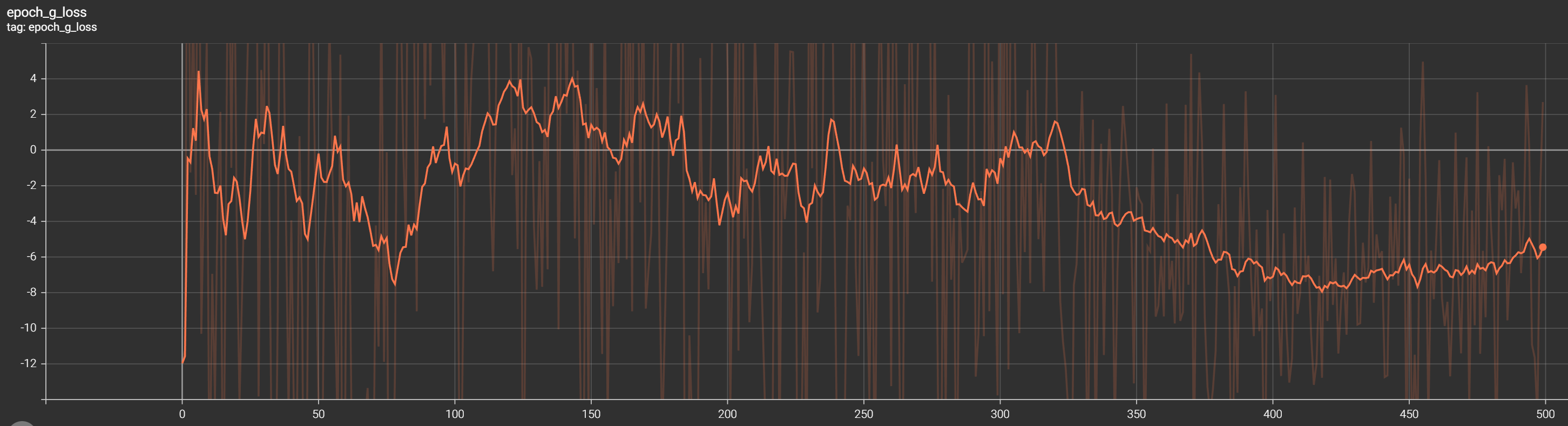
At the beginning of training, the generator loss may be low as the generator produces random samples that are easily discernible from real data. This is normal.
As training progresses, the generator loss should gradually increase, indicating that the generator is learning to generate more realistic samples that fool the discriminator.
The convergence of the generator loss depends on various factors, including the dataset, model architecture, and training hyperparameters. The generator loss is expected not to reach zero but stabilize at a certain value once it reaches its optimal performance.
In my example, we can't see where it stabilizes, but after 350 training epochs, it starts to stabilize. We would need to continue training to see better results:
Discriminator loss
Initially, the discriminator loss drops to negative rapidly first as it struggles to differentiate between real and generated samples.
As training progresses, the discriminator loss should gradually climb up, indicating that the discriminator is becoming better at distinguishing between real and generated data.
Similar to the generator loss, the discriminator loss is not expected to reach zero but should stabilize at a certain value.
That's exactly what we see in our TensorBoard discriminator curve:
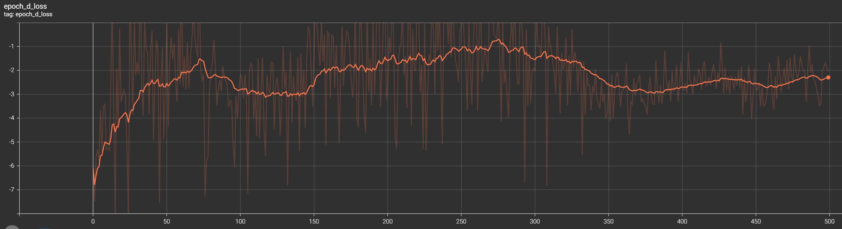
Ideally, the loss curves should converge to a relatively stable state, indicating that the generator and discriminator have reached dynamic equilibrium. The specific shape and trajectory of the loss curves can vary depending on the dataset, model architecture, and training parameters.
So, now let's look at the results from all training epochs in the following GIF:
Conclusion:
In conclusion, we have explored the limitations of the simple DCGAN architecture, specifically its training instability and the degradation in generated image quality over time. To address these issues, we introduced the Wasserstein GAN (WGAN) and its improved version, the Wasserstein GAN with Gradient Penalty (WGAN-GP).
WGAN introduced the Wasserstein loss, which addressed the instability problems associated with traditional GAN training. It carefully eliminated the need to balance the discriminator and generator and provided continuous and differentiable gradients to solve the vanishing gradient problem.
I recommend reviewing the previous tutorial on DCGAN implementation for a better understanding of the transition to WGAN-GP. We covered the necessary steps for preparing the CelebA dataset and implemented the generator and discriminator models specifically for generating 64x64 pixel-sized images of people's profiles.
We introduced a custom callback class that generated and saved images during training to track the training progress. Additionally, a learning rate scheduler was implemented to gradually decrease the learning rate over epochs for better training results.
Finally, we defined the discriminator and generator loss functions based on the Wasserstein distance, which measured the distance between real and generated data distributions.
Overall, the WGAN-GP architecture presented in this tutorial provides a more stable and effective approach to training GANs for generating high-quality images. Incorporating the Wasserstein loss and gradient penalty overcomes the limitations of the simple DCGAN architecture and produces more realistic and visually appealing results!
The complete code for this tutorial you can find in this GitHub link.
The trained model and results can be downloaded from this link.