Introduction to Reinforcement Learning Policy Gradient

Up to this moment, we covered the most popular tutorials related to DQN — value-based reinforcement learning algorithms. In deep reinforcement learning, deep Q-learning Networks are relatively simple. DQN's are comparatively simple to their credit, but many other deep RL agents also make efficient use of the training samples available. That said, DQN agents do have drawbacks. Most notable are:

1. Suppose the possible number of state-action pairs is relatively large in a given environment. In that case, the Q-function can become highly complicated, so it becomes intractable to estimate the optimal Q-value.
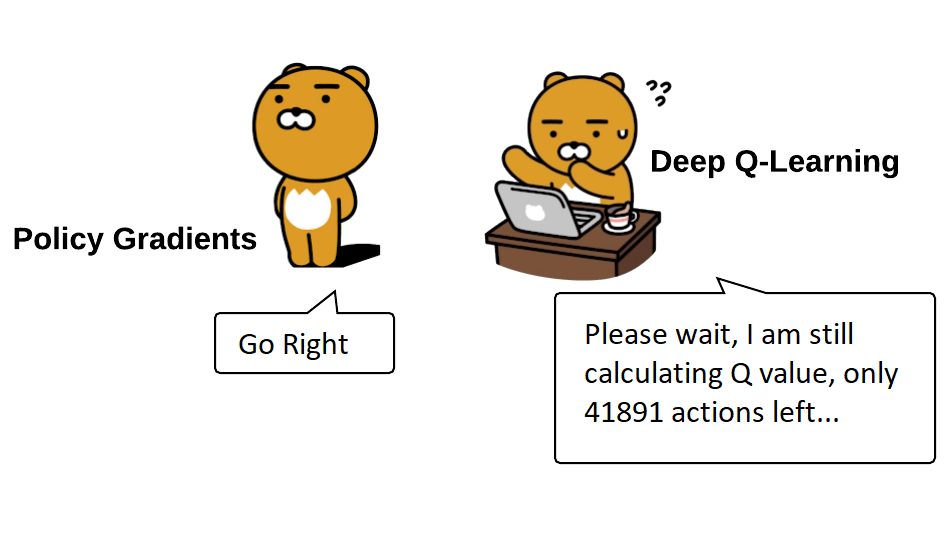
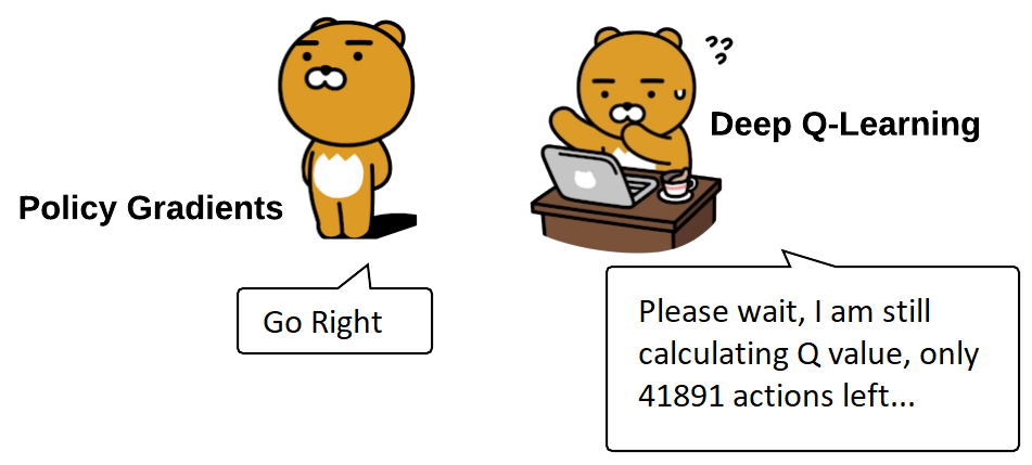
2. Even in situations where finding Q is computationally tractable, DQN's are not great at exploring relative to some other approaches, so a DQN may not work correctly.

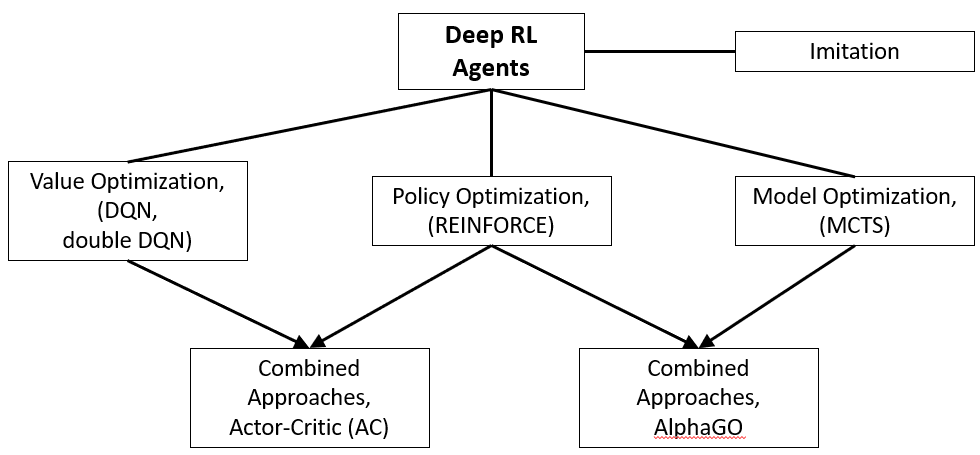
Even if DQN's are sample efficient, they don't apply to solve all problems. To wrap up deep reinforcement learning, I'll introduce the types of agents beyond DQN's (image below). The main categories of deep RL agents are:

• Value optimization: These include DQN agents and their derivatives (e.g., double DQN, dueling DQN) and other types of agents that solve reinforcement learning problems by optimizing value functions (including Q-value functions);
• Imitation learning: agents in this category (e.g., behavioral cloning and conditional imitation learning algorithms) are designed to mimic behaviors that are taught to them through demonstration, for example, showing them how to do some task, for example, pick and place boxes. Although imitation learning is a fascinating approach, its range of applications is relatively small, and I will not discuss it further;
• Model optimization: agents in this category learn to predict future states based on (s, a) at a given timestep. An example of one such algorithm is the Monte Carlo tree search (MCTS);
• Policy optimization: Agents in this category learn policies directly; they directly learn the policy function π. I'll cover these in other tutorials.

Policy Gradient and the REINFORCE Algorithm:

In DQN, we take action with the highest Q-value (maximum expected future reward at each state) to choose which action to take in each state. Therefore, value-based learning policies exist only because of these assessments of the value of the action. In this tutorial, we'll learn a policy-based reinforcement learning technique called Policy Gradients.

I already said that the Reinforcement Learning agent's primary goal is to learn some policy function π that maps the state space S to the action space A. With DQN's, and with any other value optimization agent, π is indirectly learned by estimating a value function such as the optimal Q-value. With policy optimization agents, π is learned directly instead.

This means that we are directly trying to optimize our policy function π without worrying about the value function. We'll now parameterize π (select an action without a value function).

Policy gradient (PG) algorithms, which can perform gradient ascent on π directly, exemplify a particularly well-known Reinforcement Learning algorithm called REINFORCE. The advantage of PG algorithms such as REINFORCE is that they are likely to converge with the optimal solution, so they are more widely used than value optimization algorithms such as DQN.

The trade-off is that PG has low consistency. They have a more significant difference in their performance compared to value optimization techniques such as DQN, so PGs usually require a more significant number of training samples.

In this tutorial, we'll learn:

• What is the Policy Gradient algorithm, its advantages, and disadvantages;
• How to implement it in TensorFlow 1.15 and Keras 2.2.4 (should work in TensorFlow 2 also).

Why using Policy-Based methods?

First, we will define a policy network that implements, for example, AI car drivers. This network will take the state of the car (for example, the car's velocity, the distance between the car and the track road lines) and choose what we should do (steer left or right, hit the speed pedal, or hit the brake). It's known as Policy-Based Reinforcement Learning because, as a result, we will parametrize the policy directly. Here is how our policy function will look:

${\pi }_Q(s, a)=P\left[a\right|s, Q]$

Here:
s - state value; a - action value; Q - model parameters of the policy network. We can think that policy is the agent's behavior, i.e., a function to map from state to action.

A policy can be either deterministic or stochastic. A deterministic policy is a policy that maps states to actions. We give a current state to the policy, and the function returns an action what we should take:

• Deterministic policies are used in deterministic environments. These are environments where the taken action verifies the result. There is no uncertainty. For example, when you play chess and move your pawn from A3 to A4, you're sure that your pawn will move to A4. 
  Deterministic policy: a=μ(s)
  On the other hand, a stochastic policy provides a probability distribution for actions.
• Stochastic policy means that instead of being sure of acting a (for instance, left), there is a probability we'll take a different one (in this case, 30% that we take a right). The stochastic policy is mostly used when the environment is uncertain. This process is called a Partially Observable Markov Decision Process (POMDP).
  Most of the time, we'll use this second type of policy. Stochastic policy: π(a|s)=P[a|s]

Advantages of using Policy Gradients

Policy-based methods have better convergence characteristics. The problem with value-based strategies is that they can have a significant oscillation while training. This is because the choice of action may change dramatically for an arbitrarily small change in the estimated action values.

Conversely, with a policy gradient, we tend to follow the slope to find the best parameters. We have a smooth update of our policy at every step.

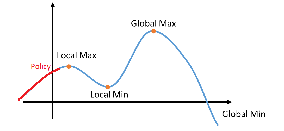
Because we tend to follow the gradient to search for the best parameters, we're guaranteed to match the local maximum (worst case) or the global maximum (best point):

The second advantage is that policy gradients are more effective in large-scale action spaces or using continuous actions.

The problem with Deep Q-learning is that their predictions assign a score (maximum expected future reward) for every possible action, within each time step, given the current state.

But what if we have endless possibilities for action? Let's take the same example, with a self-driving car, at each state, and we can have a (near) infinite choice of activities (turning the wheel at 15°, 20°, 24°, …). We will need to provide a Q value for each possible action!

On the other hand, in policy-based methods, we alter the parameters directly: Agent will start to understand what the maximum will be, instead of computing (estimating) the maximum directly at each step.

A third advantage is that policy gradient can learn a random policy, whereas value functions cannot. This has two consequences.

One of them is that we don't have to compromise and implement an exploitation/exploration trade-off. A random policy allows our agent to explore the state space without continually taking the same action. This is because it outputs a likelihood distribution over different actions. Consequently, it handles the exploration/exploitation trade-off without hard coding it.

We additionally get rid of the problem of perceptual aliasing. Perceptual aliasing is when we have two states that appear to be (or are) the same but need entirely different actions. For example, consider the game rock-paper-scissors. A deterministic policy, e.g., playing only scissors, could be easily exploited, so a random approach tends to perform much better.

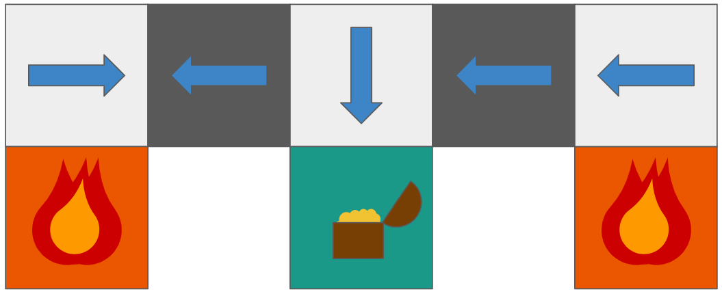
Let's take the following example. We have an intelligent gold-digger whose goal is to find the gold and avoid being killed.

Perceptual aliasing is when our agent cannot differentiate the best action to take in a state that looks very similar. Our agent sees these dark grey squares as identical states. This means that a deterministic agent would take the same action in both states.

Suppose our agent's goal is to get to the treasure whereas avoiding the fire. The two dark grey states are perceptually aliased; in different words, the agent cannot see the difference between them because they look identical. Within the case of a deterministic policy, the agent would do the same action for both of those states and would never get to the treasure. However, a random policy might move either left or right, giving it a higher probability of reaching the prize. The only hope is doing the unexpected action selected by the epsilon-greedy exploration technique.

As with Markov Decision Processes, one disadvantage of policy-based strategies is that they typically take longer to converge, and evaluating the policy requires more time. Another disadvantage is that they tend to converge to the local optimum instead of the global optimum.

Despite these pitfalls, policy gradients tend to perform better than value-based reinforcement learning agents in complex tasks. As we will see in future tutorials, several advancements in reinforcement learning when beating humans at advanced games like DOTA use techniques based on policy gradients.

Disadvantages

Naturally, Policy gradients have one major shortcoming. For a long time, they converge with the local maximum, not the global optimum. Another disadvantage of policy-based methods is that they generally take longer to converge, and evaluating the policy is time-consuming.

Instead of Deep Q-Learning, always trying to reach the maximum, the policy gradient steps gradually converge. They can take longer to train.

However, we will see that there are solutions to this problem. I already mentioned that we have our policy π that has a parameter Q. This π outputs a probability distribution of acting in a given state S with parameters theta:

${\pi }_Q(s, a)=P\left[a\right|s, Q]$

You may wonder, how do we know if our policy is good enough? Keep in mind that the policy can be seen as an optimization issue. We need to find the best parameters (Q) to maximize the score function, J(Q). There are two steps:

• We can measure the quality of a policy with a policy score function J(Q);
• We can use policy gradient ascent to find the best parameter Q that improves our policy.

The basic idea is that J (Q) will tell us how good our policy (π) is. Policy gradient ascent will help us to find the best policy parameters to maximize the example of good action.

Regardless of these pitfalls, policy gradients perform better than value-based reinforcement learning agents at complex tasks. In fact, many of the advancements in reinforcement learning beating humans at complex games such as DOTA use techniques based on policy gradients, as we’ll see in coming tutorials.

Policy Score function J(Q)

Three methods work equally well for optimizing policies. The choice depends only on the environment and the objectives we have. To measure how good our policy is, we use a function called the objective function or Policy Score Function that calculates the expected reward of the policy. In an episodic environment, we always use the start value. Then we calculate the mean of the return from the first timestep (G1), which is called the cumulative discounted reward for the entire episode:

$J_1\left(Q\right)=E_{\pi }[G_1=R_1+\gamma +{\gamma }^2{R}_3+...]=E_{\pi }\left(V\right(s_1\left)\right)$

Here:
- [G₁=R₁+γ+γ²R₃+...] - cumulative discounted reward starting at start state; E_π(V(s₁)) - the value of state 1.

The idea is simple, if we always start in some state s₁, what total reward will we get from that beginning state to the end? Losing, in the beginning, is fine, but we want to improve the outcome. For example, if we play a new game in Pong, we lose the ball in the first round. A new round always starts in the same state. We calculate the result using J₁ (Q). To do this, we will need to refine the probability distribution of my actions by adjusting the parameters.

We can use average value in a continuous environment because we cannot rely on a specific initial state. Because some states occur more than others, each state value should be weighted by the probability of the occurrence of the respected state:

$J_{avgv}\left(Q\right)=E_{\pi }\left(V\right(s\left)\right)=\sum d\left(s\right)V\left(s\right)$

Finally, we can use the average reward per step. The idea is that we want to get the maximum bonus for every stage:

$d\left(s\right)=\frac{N\left(s\right)}{\sum _{s\text{'}}N(s\text{'})}$

Here:
N(s) - Number of occurrences of the state; ∑_s'N(s') Total number occurrences of all states.

Finally, we can use the average reward per time step. The idea here is that we want to get the most reward per time step:

$J_{avR}\left(Q\right)=E_{\pi }\left(r\right)=\sum _{s}d\left(s\right)V\left(s\right)\sum _a\pi Q(s,a)R_s^a$

Here:
∑sd(s) - Probability that I am in state s; ∑aπQ(s, a) - Probability that I will take this action a from that state under this policy; R - Immediate reward that I will get.

Policy gradient ascent

We have a policy score function that tells us how good our policies are. Now we want to find the parameter Q that may maximize this score function. Maximizing the score function means finding the optimum policy.

To maximize the score function, we need to use the so-called gradient ascent on policy parameters.

Policy Gradient ascent is the inverse of the gradient descent (gradient descent always shows the steepest change). Descending the gradient, we take the direction of the sharpest decrease in the function. As we ascend the slope, we take the fastest path of function increase.

Why gradient ascent and not gradient descent? As a result, we tend to use gradient descent after having an error function that we wish to reduce.

But, keep in mind, the score function is not an error function! It is a score function, and since we wish to maximize the score, we want to use gradient ascent.

The main idea is to find the gradient of the current policy, which updates the parameters in the direction of the most significant increase and repeats.

Let's implement policy gradient ascent mathematically. This tutorial is challenging. However, it's fundamental to understand how to arrive at our gradient formula.

So, we want to find the best parameters Q* that maximize the score:

$Q*=argmax{E}_{\pi Q}\left[\sum _{t}R(s_t, a_t\right]$

Here, arguments that are after argmax, starting from E, are equal to J(Q), so our score function can be defined as:

$J\left(Q\right)=E_{\pi }\left[T\right(\tau \left)\right]$

Here:
E - expected given policy; τ - Expected future reward.

The above formula shows us the total summation of the expected reward with a given policy. Now, we need to do gradient ascent to differentiate our score function J(Q). Our score function J(Q) can also be defined as:

$J_1\left(Q\right)=V_{\pi Q}\left(s1\right)=E_{\pi Q}=\sum _{a\ni S}d\left(s\right)\sum _{a\ni A}{\pi }_Q(S, a)R_s^a$

I wrote the function this way to show the problem we are facing here. We know that policy parameters change the way actions are chosen, and, as a result, we receive the rewards that states will see and how often.

Thus, it's going to be not very easy to seek out policy changes to ensure improvement. This is because performance depends on the choices of actions and the distribution of the states in which those choices are made.

Both are affected by policy parameters. The impact of policy parameters on actions is easy to find, but how to find the impact of policy on the distribution of the state? The environment function is unknown. As a result, we face a problem: how to estimate ∇ (gradient) concerning policy Q when the gradient depends on the unknown effect of policy changes on the state distribution?

The solution to the above problem is to use the Policy Gradient theorem. This provides an analytical expression for the J (Q) (activity) gradient concerning the policy Q, which does not imply a differentiation of the state distribution.

So continuing calculating the above J(Q) expression, we can write:

${\nabla }_{Q}J\left(Q\right)={\nabla }_Q\sum _{\tau }\pi (\tau ; Q)R\left(\tau \right)$

Now, we're in a situation of stochastic policy. We'll put the gradient inside the above formula instead of everything up to R(τ). This means that our approach provides a probability distribution π(τ; Q). Given our current parameters Q, the probability of performing these steps (s0, a0, r0, …) is obtained.

But it isn't easy to separate the probability function unless we can turn it into a logarithm. This makes it much easier to distinguish. Thus, we will use a probability ratio trick that will convert the resulting part into log probability. The probability ratio trick looks like this:

$\nabla \log x=\frac{\nabla x}{x}$

From the above expression, we can write:

$\pi (\tau ; Q)\frac{{\nabla }_Q\pi (\tau ; Q)}{\pi (\tau ; Q)}$

With the above expression, we can get the following expression:

$\sum _{\tau }\pi (\tau ; Q)={\nabla }_Q\left(\log \pi \right(\tau ; Q\left)\right)R\left(\tau \right)$

Finally, we can convert the summation back to expectation:

${\nabla }_{Q}J\left(Q\right)=E_{\pi }\left[{\nabla }_Q\right(\log \pi (\tau ; Q)\left)R\right(\tau \left)\right]$

Here:
π(τ|Q) - Policy function; R(τ) - Score function.

As you can see, we only need to calculate the derivative of the log policy function. Now that we've done that, and it was a lot, we can conclude about policy gradients:

$E_{\pi }\left[{\nabla }_Q\right(\log \pi (s, a, Q)\left)R\right(\tau \left)\right]$

Here:
π(s,a,Q) - Policy function; R(τ) - Score function.

And our Update rule looks like this:

$∆Q=a*{\nabla }_Q\left(\log \pi \right(s, a, Q\left)\right)R\left(\tau \right)$

Here:
△Q - Change in parameters; α - Learning rate.

This Policy gradient tells us how we should shift the policy distribution by changing parameters Q to achieve a higher score.

R(τ) is like a scalar value score:

• If R(τ) is high, it means that we took actions that led to high rewards on average. We want to accelerate the likelihood of visible actions (increase the possibility of these actions being performed).
• On the other hand, if R (τ) is small, we want to displace the probability of seen action.

In simple terms, the policy is the mindset of the agent. The agent sees the current situation (state) and chooses to choose an action. (or multiple actions) so we define policy as a function of the state that outputs some actions: action=f(state) we call the above f function policy gradient policy.

Reward Engineering and why it is important

One of the essential things in all policy gradient agents is how we work with reward. From reward, function depends on how good our Model will be learning. This is an example, how our rewards would look in our pong game:

[0.0, 0.0, 0.0, 0.0, 0.0, 0.0, 0.0, 0.0, 0.0, 0.0, 0.0, 0.0, 0.0, 0.0, 0.0, 0.0, 0.0, 0.0, 0.0, 0.0, 0.0, 0.0, 0.0, 0.0, 0.0, 0.0, 0.0, 0.0, 0.0, 0.0, 0.0, 0.0, 0.0, -1.0, 0.0, 0.0, 0.0, 0.0, 0.0, 0.0, 0.0, 0.0, 0.0, 0.0, 0.0, 0.0, 0.0, 0.0, 0.0, 0.0]

So the rewards are mostly zero, and sometimes we may see 1 or -1 on the list. This is because the environment gives us a bonus when the ball passes through an opponent or us. When the ball passes our paddle, we lose and get a -1 reward, and when the opponent fails to catch the ball, we win and get +1.

If we train our network with this reward, it learns nothing because the reward is most of the time zero. In this case, the agent does not get feedback on what is good or bad. Most gradients would become zero because reward multiplication is used in the loss function. Environment rewards us just when the ball passes through our paddle (we score -1) or our opponent's paddle(we score +1).

Now think about it:

Our paddle moves up and down, hits the ball, and travels to the screen's left side. The opponent fails to catch it, and we win and get a score of one. In this scenario, which actions were good?

1. The action we took when we hit the ball?
2. The action we took when we got a score of 1?

Of course, the first option is correct. The second option is wrong because our action does not matter when the ball is reaching the opponent. Only the action that we took to hit the ball was important to winning. Everything after hitting the ball was irrelevant to our win. (a somewhat similar argument can be discussed losing the actions near when we got a score of -1 is more critical than actions taken many steps earlier).

So here is the trick. We set the reward of actions taken before each reward, similar to the reward obtained. For example, if we got a reward +1 at time 200, we say that reward of time 199 is +0.99, the reward of time 198 is +0.98, and so on. With this reward definition, we have the rewards for actions that resulted in a +1 or -1. We assume the more recent the action to the reward gained, the more critical it is.

We define a function below that does this for us. Note that this may not be applicable in other environments but serves our purposes for this Pong game project.

def discount_rewards(self, reward):
    # Compute the gamma-discounted rewards over an episode
    gamma = 0.99    # discount rate
    running_add = 0
    discounted_r = np.zeros_like(reward)
    for i in reversed(range(0,len(reward))):
        if reward[i] != 0:
            running_add = 0 # (pong specific game boundary!)
        running_add = running_add * gamma + reward[i]
        discounted_r[i] = running_add

    return discounted_r

Let's see what this gives us:

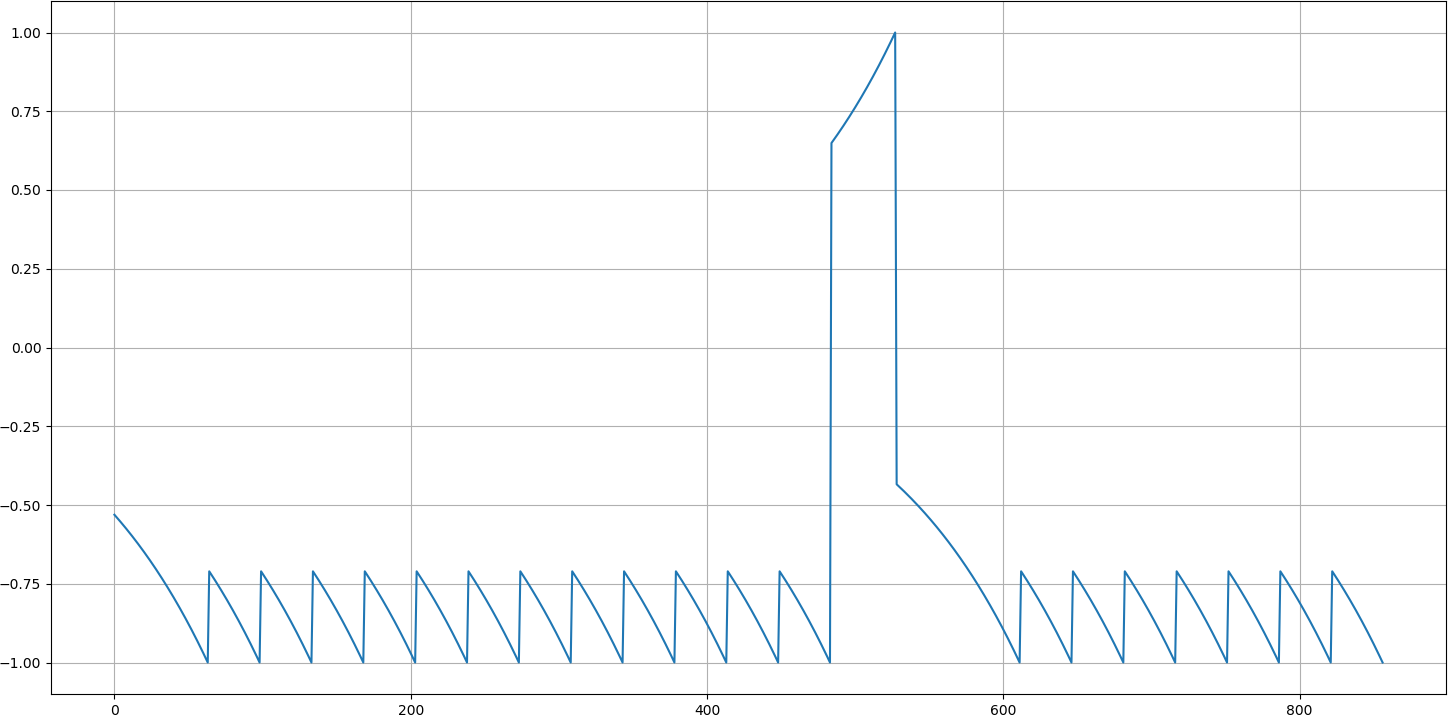
You can see that in the above chart we got better distribution for rewards. The reward is -1 where it was -1 and now steps, before it has some value near -1 (for example -0.8) and similar process, happens for positive rewards.

Furthermore, we refine the function to subtract rewards by mean and divide by std and then discuss the results.

def discount_rewards(self, reward):
    # Compute the gamma-discounted rewards over an episode
    gamma = 0.99    # discount rate
    running_add = 0
    discounted_r = np.zeros_like(reward)
    for i in reversed(range(0,len(reward))):
        if reward[i] != 0:
            running_add = 0 # (pong specific game boundary!)
        running_add = running_add * gamma + reward[i]
        discounted_r[i] = running_add

    discounted_r -= np.mean(discounted_r) # normalizing the result
    discounted_r /= np.std(discounted_r) # divide by standard deviation
    return discounted_r

Let's see our reformatted rewards:

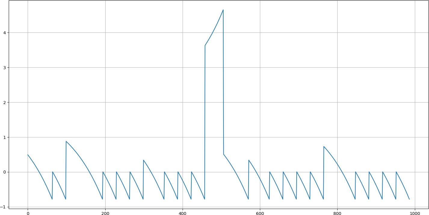So now we have rewards bigger than -0.9 most of the time.

In points where we got a -1 reward, the new score is about -0.9, as seen above, and the steps before also have negative rewards. The negativity of the reward goes down as we go to the left from each -0.9 score.

Also, you can see that we got some positive scores in our new chart. This is because we subtracted by mean. Think about what it can result in?

The positive reward happens in the long sequences of playing. These are situations where we caught the ball and didn't get a -1 immediately, but we lost later because we failed to catch the ball when it came toward us.

Setting a negative score is logical because we ended up getting a -1. Developing a positive score could be justified by approving actions where we catch the ball and did not get a -1 reward immediately (maybe we didn't win either).

At some point, you can see that even when we didn't receive a positive score, some hills were higher than others. This is because our agent succeeded in surviving longer than usual. This also helps for learning. So now that we have defined our rewards, we can go to the next step and start training the network.

Policy Gradient implementation with Pong:

So, it was quite a long theoretical tutorial, and it's usually hard to understand everything with plain text, so let's do this with a basic Pong example and implement it in Keras. Different from my previous tutorials, I will try the 'PongDeterministic-v4' environment and 'Pong-v0'. 'PongDeterministic-v4' is easier to learn, so if our Model can understand this simpler environment, we will try 'Pong-v0'. You may ask why it's simpler if it's the same pong game. A deterministic game gives us all game frames, 'Pong-v0' gives us every 4th frame, which means it is four times faster, much harder to learn playing it.

I used code from my previous DQN tutorial and rewrote it to Policy Gradient. I am not writing all details here. If you want to see all details, check my above YouTube tutorial.

Also, I am not using convolutional layers because it's quite an austere environment. It's faster to train models without CNN.

Complete code you can find on GitHub.

# Tutorial by www.pylessons.com
# Tutorial written for - Tensorflow 1.15, Keras 2.2.4

import os
import random
import gym
import pylab
import numpy as np
from keras.models import Model, load_model
from keras.layers import Input, Dense, Lambda, Add, Conv2D, Flatten
from keras.optimizers import Adam, RMSprop
from keras import backend as K
import cv2

def OurModel(input_shape, action_space, lr):
    X_input = Input(input_shape)

    #X = Conv2D(32, 8, strides=(4, 4),padding="valid", activation="elu", data_format="channels_first", input_shape=input_shape)(X_input)
    #X = Conv2D(64, 4, strides=(2, 2),padding="valid", activation="elu", data_format="channels_first")(X)
    #X = Conv2D(64, 3, strides=(1, 1),padding="valid", activation="elu", data_format="channels_first")(X)
    X = Flatten(input_shape=input_shape)(X_input)

    X = Dense(512, activation="elu", kernel_initializer='he_uniform')(X)
    #X = Dense(256, activation="elu", kernel_initializer='he_uniform')(X)
    #X = Dense(64, activation="elu", kernel_initializer='he_uniform')(X)

    action = Dense(action_space, activation="softmax", kernel_initializer='he_uniform')(X)

    Actor = Model(inputs = X_input, outputs = action)
    Actor.compile(loss='categorical_crossentropy', optimizer=RMSprop(lr=lr))

    return Actor

class PGAgent:
    # Policy Gradient Main Optimization Algorithm
    def __init__(self, env_name):
        # Initialization
        # Environment and PG parameters
        self.env_name = env_name       
        self.env = gym.make(env_name)
        self.action_size = self.env.action_space.n
        self.EPISODES, self.max_average = 10000, -21.0 # specific for pong
        self.lr = 0.000025

        self.ROWS = 80
        self.COLS = 80
        self.REM_STEP = 4

        # Instantiate games and plot memory
        self.states, self.actions, self.rewards = [], [], []
        self.scores, self.episodes, self.average = [], [], []

        self.Save_Path = 'Models'
        self.state_size = (self.REM_STEP, self.ROWS, self.COLS)
        self.image_memory = np.zeros(self.state_size)
        
        if not os.path.exists(self.Save_Path): os.makedirs(self.Save_Path)
        self.path = '{}_PG_{}'.format(self.env_name, self.lr)
        self.Model_name = os.path.join(self.Save_Path, self.path)

        # Create Actor network model
        self.Actor = OurModel(input_shape=self.state_size, action_space = self.action_size, lr=self.lr)

    def remember(self, state, action, reward):
        # store episode actions to memory
        self.states.append(state)
        action_onehot = np.zeros([self.action_size])
        action_onehot[action] = 1
        self.actions.append(action_onehot)
        self.rewards.append(reward)

    def act(self, state):
        # Use the network to predict the next action to take, using the model
        prediction = self.Actor.predict(state)[0]
        action = np.random.choice(self.action_size, p=prediction)
        return action

    def discount_rewards(self, reward):
        # Compute the gamma-discounted rewards over an episode
        gamma = 0.99    # discount rate
        running_add = 0
        discounted_r = np.zeros_like(reward)
        for i in reversed(range(0,len(reward))):
            if reward[i] != 0: # reset the sum, since this was a game boundary (pong specific!)
                running_add = 0
            running_add = running_add * gamma + reward[i]
            discounted_r[i] = running_add

        discounted_r -= np.mean(discounted_r) # normalizing the result
        discounted_r /= np.std(discounted_r) # divide by standard deviation
        return discounted_r

    def replay(self):
        # reshape memory to appropriate shape for training
        states = np.vstack(self.states)
        actions = np.vstack(self.actions)

        # Compute discounted rewards
        discounted_r = self.discount_rewards(self.rewards)

        # training PG network
        self.Actor.fit(states, actions, sample_weight=discounted_r, epochs=1, verbose=0)
        # reset training memory
        self.states, self.actions, self.rewards = [], [], []
    
    def load(self, Actor_name):
        self.Actor = load_model(Actor_name, compile=False)

    def save(self):
        self.Actor.save(self.Model_name + '.h5')

    pylab.figure(figsize=(18, 9))
    def PlotModel(self, score, episode):
        self.scores.append(score)
        self.episodes.append(episode)
        self.average.append(sum(self.scores[-50:]) / len(self.scores[-50:]))
        if str(episode)[-2:] == "00":# much faster than episode % 100
            pylab.plot(self.episodes, self.scores, 'b')
            pylab.plot(self.episodes, self.average, 'r')
            pylab.ylabel('Score', fontsize=18)
            pylab.xlabel('Steps', fontsize=18)
            try:
                pylab.savefig(self.path+".png")
            except OSError:
                pass

        return self.average[-1]

    def imshow(self, image, rem_step=0):
        cv2.imshow(self.Model_name+str(rem_step), image[rem_step,...])
        if cv2.waitKey(25) & 0xFF == ord("q"):
            cv2.destroyAllWindows()
            return

    def GetImage(self, frame):
        # croping frame to 80x80 size
        frame_cropped = frame[35:195:2, ::2,:]
        if frame_cropped.shape[0] != self.COLS or frame_cropped.shape[1] != self.ROWS:
            # OpenCV resize function 
            frame_cropped = cv2.resize(frame, (self.COLS, self.ROWS), interpolation=cv2.INTER_CUBIC)
        
        # converting to RGB (numpy way)
        frame_rgb = 0.299*frame_cropped[:,:,0] + 0.587*frame_cropped[:,:,1] + 0.114*frame_cropped[:,:,2]

        # convert everything to black and white (agent will train faster)
        frame_rgb[frame_rgb < 100] = 0
        frame_rgb[frame_rgb >= 100] = 255
        # converting to RGB (OpenCV way)
        #frame_rgb = cv2.cvtColor(frame_cropped, cv2.COLOR_RGB2GRAY)     

        # dividing by 255 we expresses value to 0-1 representation
        new_frame = np.array(frame_rgb).astype(np.float32) / 255.0

        # push our data by 1 frame, similar as deq() function work
        self.image_memory = np.roll(self.image_memory, 1, axis = 0)

        # inserting new frame to free space
        self.image_memory[0,:,:] = new_frame

        # show image frame   
        #self.imshow(self.image_memory,0)
        #self.imshow(self.image_memory,1)
        #self.imshow(self.image_memory,2)
        #self.imshow(self.image_memory,3)
        return np.expand_dims(self.image_memory, axis=0)

    def reset(self):
        frame = self.env.reset()
        for i in range(self.REM_STEP):
            state = self.GetImage(frame)
        return state

    def step(self,action):
        next_state, reward, done, info = self.env.step(action)
        next_state = self.GetImage(next_state)
        return next_state, reward, done, info
    
    def run(self):
        for e in range(self.EPISODES):
            state = self.reset()
            done, score, SAVING = False, 0, ''
            while not done:
                #self.env.render()
                # Actor picks an action
                action = self.act(state)
                # Retrieve new state, reward, and whether the state is terminal
                next_state, reward, done, _ = self.step(action)
                # Memorize (state, action, reward) for training
                self.remember(state, action, reward)
                # Update current state
                state = next_state
                score += reward
                if done:
                    average = self.PlotModel(score, e)
                    # saving best models
                    if average >= self.max_average:
                        self.max_average = average
                        self.save()
                        SAVING = "SAVING"
                    else:
                        SAVING = ""
                    print("episode: {}/{}, score: {}, average: {:.2f} {}".format(e, self.EPISODES, score, average, SAVING))

                    self.replay()
        
        # close environemnt when finish training
        self.env.close()

    def test(self, Model_name):
        self.load(Model_name)
        for e in range(100):
            state = self.reset()
            done = False
            score = 0
            while not done:
                self.env.render()
                action = np.argmax(self.Actor.predict(state))
                state, reward, done, _ = self.step(action)
                score += reward
                if done:
                    print("episode: {}/{}, score: {}".format(e, self.EPISODES, score))
                    break
        self.env.close()

if __name__ == "__main__":
    env_name = 'Pong-v0'
    #env_name = 'PongDeterministic-v4'
    agent = PGAgent(env_name)
    #agent.run()
    #agent.test('Models/PongDeterministic-v4_PG_2.5e-05.h5')
    agent.test('Models/Pong-v0_PG_2.5e-05.h5')

So, I trained 'PongDeterministic-v4' for 1000 steps, results you can see in bellow graph:

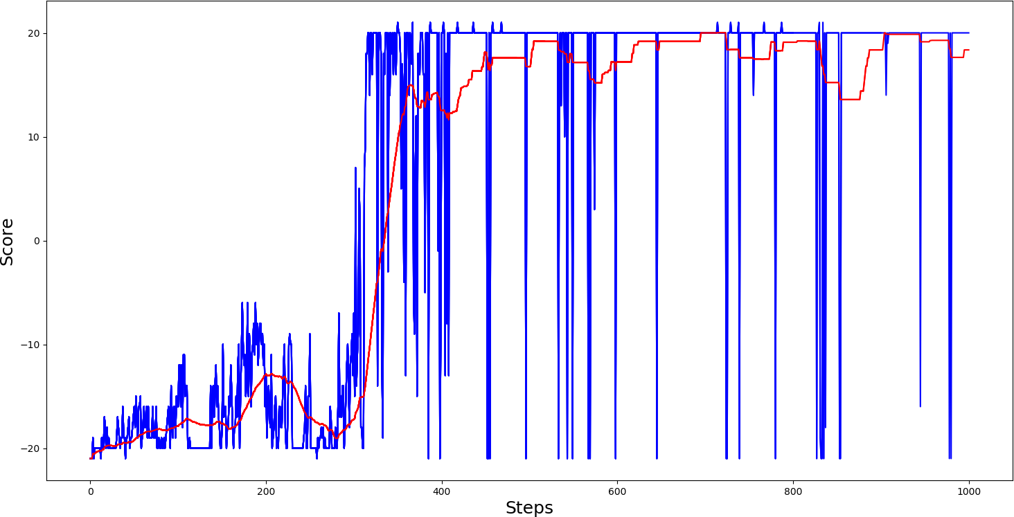This training graph shows that our Model reached an average score of 20 somewhere around the 700th step, quite nice. I also trained the 'Pong-v0' model. Here is how it performed:

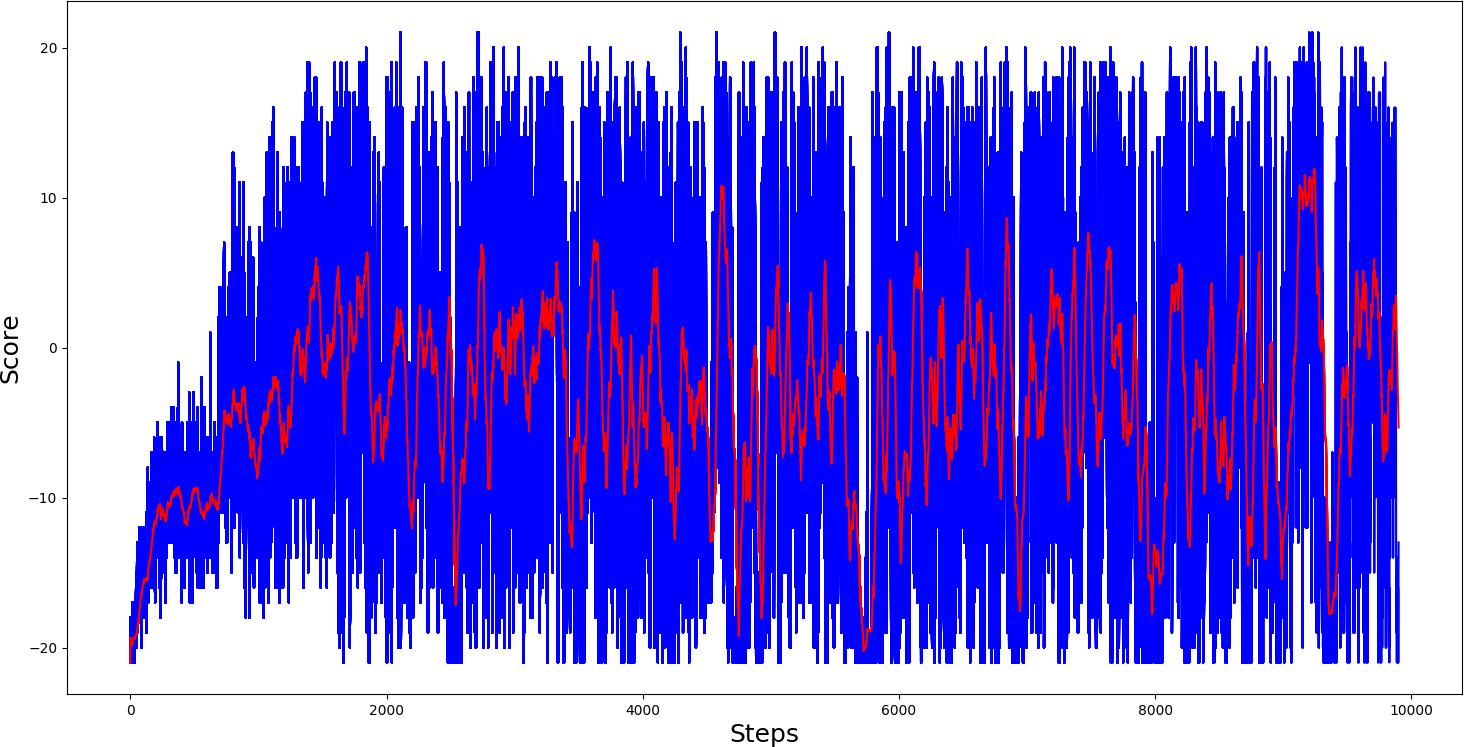Looking at the graph above, we can see that our agent learned to play Pong, but it was precarious. Although it plays pong much better than random agent testing, this Model would perform quite severely.

As you can see, the Policy Gradient model learned to play and score some points. I made our Model of one deep layer because of simplicity, I didn't want to make the perfect agent, but if you wish, you can try and train the network a lot more to play better. You can try playing around with CNN, but then you would need to decrease the learning rate, but as a result, you will get a smaller model because now the Model takes around 100 MB of size, so I can't upload a trained model to GitHub.

Conclusion:

However, from this tutorial code, we face a problem with this algorithm. Since we only calculate reward at the end of the episode, we evaluate and average all actions. Even if some of the actions taken were very bad, we would rate all the actions as good if our score is relatively high.

So to have the right policies, we need many samples, which leads to slow learning.

How to improve our Model? We'll see in the next tutorials some improvements:

• Actor-Critic: a hybrid between value-based algorithms and policy-based algorithms;
• Proximal Policy Gradients: ensures that deviations from previous policies remain relatively small.