Logistic Regression cost optimization function

Let's begin with steps we defined in the previous tutorial and what's left to do:

• Define the model structure (data shape) (done);
• Initialize model parameters;
• Learn the parameters for the model by minimizing the cost:
  - Calculate current loss (forward propagation) (done);
  - Calculate current gradient (backward propagation) (done);
  - Update parameters (gradient descent);
• Use the learned parameters to make predictions (on the test set);
• Analyse the results and conclude the tutorial.

In the previous tutorial, we defined our model structure, learned to compute a cost function and its gradient. In this tutorial, we will write an optimization function to update the parameters using gradient descent.

So we'll write the optimization function that will learn w and b by minimizing the cost function J. For a parameter θ, the update rule is (α is the learning rate):

$\theta =\theta -\alpha d\theta$

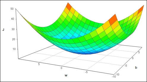
The cost function in logistic regression:

One of the reasons we use the cost function for logistic regression is that it’s a convex function with a single global optimum. You can imagine rolling a ball down the bowl-shaped function (image bellow)  -  it would settle at the bottom.

Similarly, to find the minimum cost function, we need to get to the lowest point. To do that, we can start from anywhere on the function and iteratively move down in the direction of the steepest slope, adjusting the values of w and b that lead us to the minimum. For this, we use the following two formulas:

$$\begin{gathered} w=w-\alpha \frac{\partial J(w, b)}{\partial w} \\ b=b-\alpha \frac{\partial J(w, b)}{\partial b} \end{gathered}$$

In these two equations, the partial derivatives dw and db represent the effect that a change in w and b have on the cost function, respectively. By finding the slope and taking the negative of that slope, we ensure that we will always move in the minimum direction. To get a better understanding, let’s see this graphically for dw:

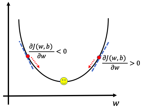
When the derivative term is positive, we move in the opposite direction towards a decreasing value of w. When the derivative is negative, we move toward increasing w, thereby ensuring that we’re always moving toward the minimum.

The alpha term in front of the partial derivative is called the learning rate and measures how big a step to take at each iteration. The choice of learning parameters is an important one - too small, and the model will take very long to find the minimum, too large, and the model might overshoot the minimum and fail to find the minimum.

Gradient descent is the essence of the learning process - through it, the machine learns what values of weights and biases minimize the cost function. It does this by iteratively comparing its predicted output for a set of data to the true output in the training process.

Coding optimization function:

So we will implement an optimization function, but first, let's see what are the inputs and outputs to it:

Arguments:

w - weights, a NumPy array of size (ROWS * COLS * CHANNELS, 1);
b - bias, a scalar;
X - data of size (ROWS * COLS * CHANNELS, number of examples);
Y - true "label" vector (containing 0 if a dog, 1 if cat) of size (1, number of examples);
num_iterations - number of iterations of the optimization loop;
learning_rate - learning rate of the gradient descent update rule;
print_cost - True to print the loss every 100 steps.

Return:

params - a dictionary containing the weights w and bias b;
grads - a dictionary containing the gradients of the weights and bias concerning the cost function;
costs - list of all the costs computed during the optimization.

Here is the code:

def optimize(w, b, X, Y, num_iterations, learning_rate, print_cost = False):
    costs = []    
    for i in range(num_iterations):
        # Cost and gradient calculation
        grads, cost = propagate(w, b, X, Y)
        
        # Retrieve derivatives from grads
        dw = grads["dw"]
        db = grads["db"]

        # update w and b
        w = w - learning_rate*dw
        b = b - learning_rate*db

        # Record the costs
        if i % 100 == 0:
            costs.append(cost)
            
        # Print the cost every 100 training iterations
        if print_cost and i % 100 == 0:
            print ("Cost after iteration %i: %f" %(i, cost))

    # update w and b to dictionary
    params = {"w": w,
              "b": b}
    
    # update derivatives to dictionary
    grads = {"dw": dw,
             "db": db}
    
    return params, grads, costs

Let's test the above function with variables from our previous tutorial where we were writing propogate() function:

params, grads, costs = optimize(w, b, X, Y, num_iterations = 100, learning_rate = 0.009, print_cost = False)

print("w = " + str(params["w"]))
print("b = " + str(params["b"]))
print("dw = " + str(grads["dw"]))
print("db = " + str(grads["db"]))

If everything is fine as a result, you should get:

w = [[-0.49157334]
 [-0.16017651]]
b = 3.948381664135624
dw = [[ 0.03602232]
 [-0.02064108]]
db = -0.01897084202791005

Full tutorial code:

import os
import cv2
import numpy as np
import matplotlib.pyplot as plt
import scipy

ROWS = 64
COLS = 64
CHANNELS = 3

TRAIN_DIR = 'Train_data/'
TEST_DIR = 'Test_data/'

#train_images = [TRAIN_DIR+i for i in os.listdir(TRAIN_DIR)]
#test_images =  [TEST_DIR+i for i in os.listdir(TEST_DIR)]

def read_image(file_path):
	img = cv2.imread(file_path, cv2.IMREAD_COLOR)
	return cv2.resize(img, (ROWS, COLS), interpolation=cv2.INTER_CUBIC)

def prepare_data(images):
	m = len(images)
	X = np.zeros((m, ROWS, COLS, CHANNELS), dtype=np.uint8)
	y = np.zeros((1, m))
	for i, image_file in enumerate(images):
		X[i,:] = read_image(image_file)
		if 'dog' in image_file.lower():
			y[0, i] = 1
		elif 'cat' in image_file.lower():
			y[0, i] = 0
	return X, y

def sigmoid(z):
	s = 1/(1+np.exp(-z))
	return s

def propagate(w, b, X, Y):
    m = X.shape[1]
    
     # FORWARD PROPAGATION (FROM X TO COST)
    z = np.dot(w.T, X)+b # tag 1
    A = sigmoid(z) # tag 2                                    
    cost = (-np.sum(Y*np.log(A)+(1-Y)*np.log(1-A)))/m # tag 5
    
    # BACKWARD PROPAGATION (TO FIND GRAD)
    dw = (np.dot(X,(A-Y).T))/m # tag 6
    db = np.average(A-Y) # tag 7

    cost = np.squeeze(cost)
    grads = {"dw": dw,
             "db": db}
    
    return grads, cost

w = np.array([[1.],[2.]])
b = 4.
X = np.array([[5., 6., -7.],[8., 9., -10.]])
Y = np.array([[1,0,1]])
'''
grads, cost = propagate(w, b, X, Y)
print(grads["dw"])
print(grads["db"])
print(cost)

train_set_x, train_set_y = prepare_data(train_images)
test_set_x, test_set_y = prepare_data(test_images)

train_set_x_flatten = train_set_x.reshape(train_set_x.shape[0], ROWS*COLS*CHANNELS).T
test_set_x_flatten = test_set_x.reshape(test_set_x.shape[0], -1).T

print("train_set_x shape " + str(train_set_x.shape))
print("train_set_x_flatten shape: " + str(train_set_x_flatten.shape))
print("train_set_y shape: " + str(train_set_y.shape))
print("test_set_x shape " + str(test_set_x.shape))
print("test_set_x_flatten shape: " + str(test_set_x_flatten.shape))
print("test_set_y shape: " + str(test_set_y.shape))

train_set_x = train_set_x_flatten/255
test_set_x = test_set_x_flatten/255
'''
def optimize(w, b, X, Y, num_iterations, learning_rate, print_cost = False):
    costs = []    
    for i in range(num_iterations):
        # Cost and gradient calculation
        grads, cost = propagate(w, b, X, Y)
        
        # Retrieve derivatives from grads
        dw = grads["dw"]
        db = grads["db"]

        # update w and b
        w = w - learning_rate*dw
        b = b - learning_rate*db

        # Record the costs
        if i % 100 == 0:
            costs.append(cost)
            
        # Print the cost every 100 training iterations
        if print_cost and i % 100 == 0:
            print ("Cost after iteration %i: %f" %(i, cost))

    # update w and b to dictionary
    params = {"w": w,
              "b": b}
    
    # update derivatives to dictionary
    grads = {"dw": dw,
             "db": db}
    
    return params, grads, costs

params, grads, costs = optimize(w, b, X, Y, num_iterations = 100, learning_rate = 0.009, print_cost = False)

print("w = " + str(params["w"]))
print("b = " + str(params["b"]))
print("dw = " + str(grads["dw"]))
print("db = " + str(grads["db"]))