One hidden layer Neural Network architecture

Welcome to another tutorial. In the last tutorial series, we wrote a logistic regression function. Now it's time to build our first neural network, which will have one hidden layer. You will see no big difference between this model and the one we implemented using logistic regression.

• Define the model structure (data shape);
• Initialize model parameters;
• Create a loop to:
  • Implement forward propagation;
  • Compute loss;
  • Implement backward propagation to get the gradients;
  • Update parameters (gradient descent)

We often build helper functions to compute 3 first steps and then merge them into one function we will call nn_model(). Once we have built nn_model() and learned the right parameters, we'll make predictions.

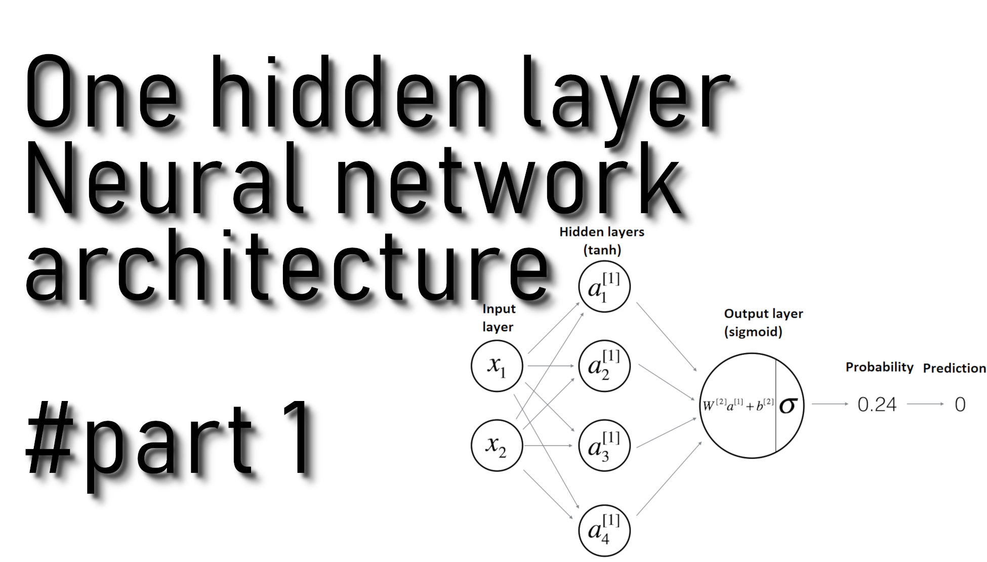
Model architecture:

You would agree that we can't get good results with Logistic Regression, we can train our model as long as we want, but it won't improve. So we going to train a Neural Network with a single hidden layer: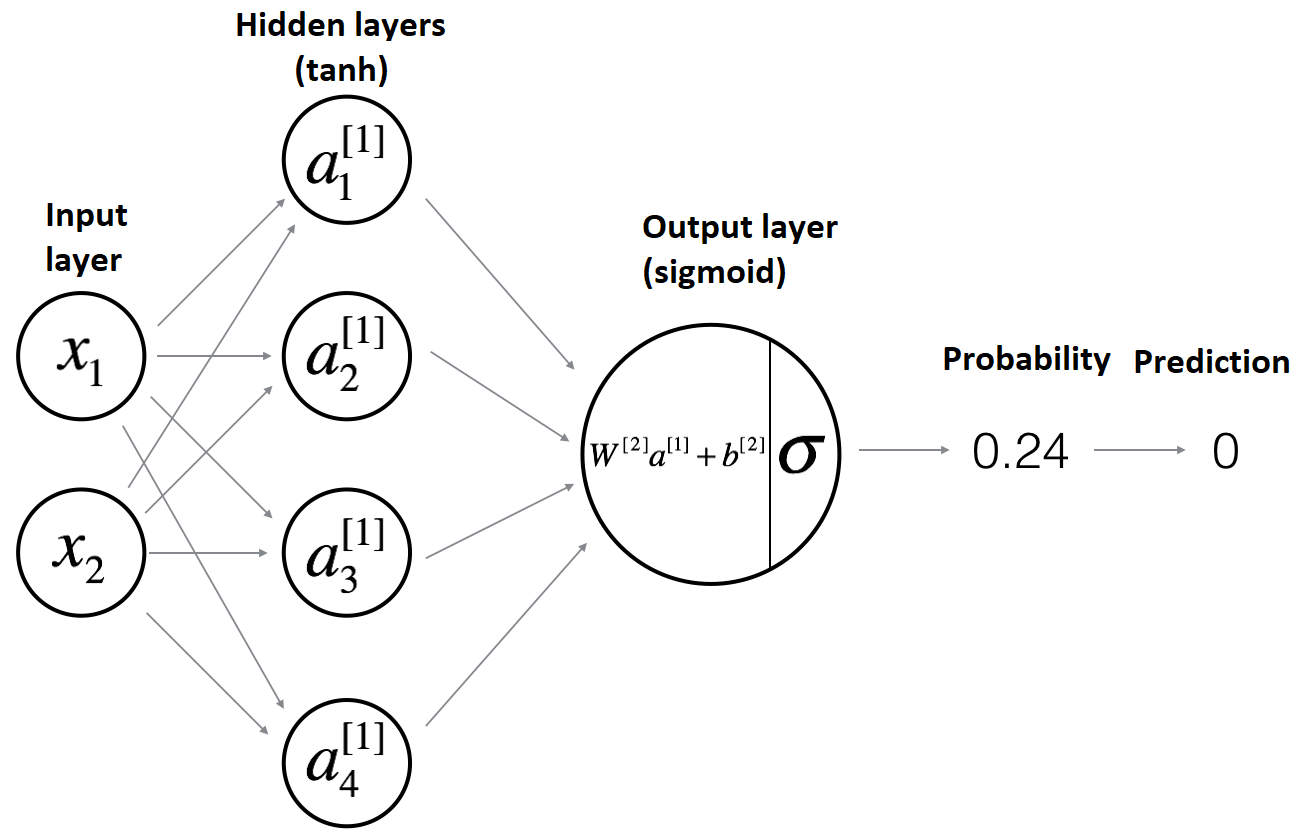

The mathematical expression of the forward propagation algorithm for one example x(i):

$$\begin{gathered} z^{\left[1\right]\left(i\right)}=W^{\left[1\right]}{x}^{\left(i\right)}+b^{\left[1\right]} \\ {a}^{\left[1\right]\left(i\right)}=\tan h\left(z^{\left[1\right]\left(i\right)}\right) \\ {z}^{\left[2\right]\left(i\right)}=W^{\left[2\right]}{x}^{\left[1\right]\left(i\right)}+b^{\left[2\right]} \\ \hat{y}=a^{\left[2\right]\left(i\right)}=\sigma \left(z^{\left[2\right]\left(i\right)}\right) \\ {y}_{prediction}^{\left(i\right)}=\left\{\begin{array}{ll}1& if a^{\left[2\right]\left(i\right)}>0.5\\ 0& otherwise\end{array}\right. \end{gathered}$$

And our final forward propagation cost function will look like this:

$J=-\frac{1}{m}\sum _{i=1}^m\left(y^{\left(i\right)}\log \left(a^{\left[2\right]\left(i\right)}\right)-(1-y^{\left(i\right)})\log (1-a^{\left[2\right]\left(i\right)})\right)$

Initialize the model's parameters:

Now, while we'll have one hidden layer in our model, we'll need to initialize parameters for input and hidden layers. Now our parameters can't be zeros from the start because hidden layer parameters depend on input layers, so we initialize them as minimal random numbers. If our weight were zeros, they would be all with the same value in every training iteration, but when we initialize them as different random numbers, they train differently. But bias can be zeros:

def initialize_parameters(input_layer, hidden_layer, output_layer):
    # initialize 1st layer output and input with random values
    W1 = np.random.randn(hidden_layer, input_layer) * 0.01
    # initialize 1st layer output bias
    b1 = np.zeros((hidden_layer, 1))
    # initialize 2nd layer output and input with random values
    W2 = np.random.randn(output_layer, hidden_layer) * 0.01
    # initialize 2nd layer output bias
    b2 = np.zeros((output_layer,1))
    
    parameters = {"W1": W1,
                  "b1": b1,
                  "W2": W2,
                  "b2": b2}
    
    return parameters

Before computing forward propagation, we'll cover tanh function.

Same as in our logistic regression, where we visualized our sigmoid and sigmoid_derivative functions and generated data from -10 to 10, we'll use the same code for our tanh visualization. Below is the full code used to print tanh and tanh_derivative functions:

from matplotlib import pylab
import pylab as plt
import numpy as np

def tanh_derivative(x):
    ds = 1 - np.power(np.tanh(x), 2)
    return ds

# linespace generate an array from start and stop value, 100 elements
values = plt.linspace(-10,10,100)

# prepare the plot, associate the color r(ed) or b(lue) and the label 
plt.plot(values, np.tanh(values), 'r')
plt.plot(values, tanh_derivative(values), 'b')

# Draw the grid line in background.
plt.grid()

# Title & Subtitle
plt.title('Sigmoid and Sigmoid derivative functions')

# plt.plot(x)
plt.xlabel('X Axis')
plt.ylabel('Y Axis')

# create the graph
plt.show()

As a result, we'll receive the following graph:

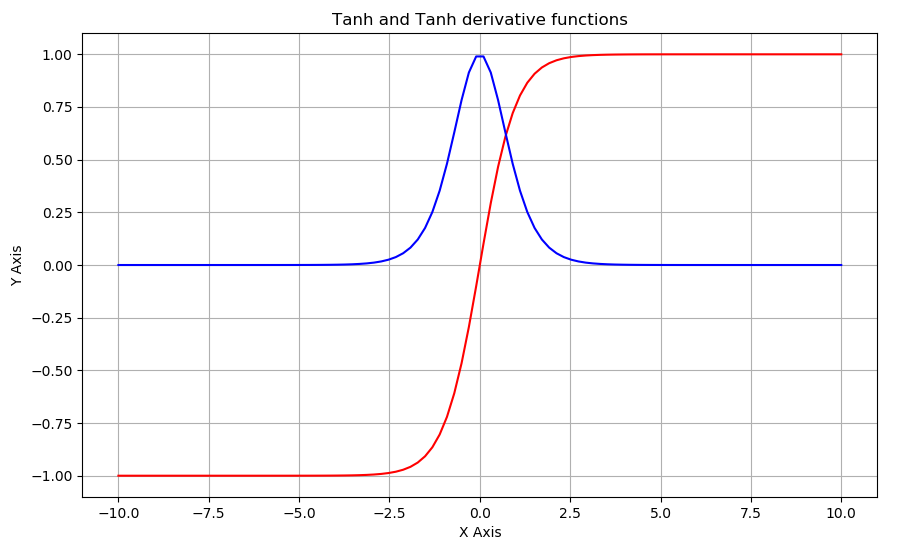
The above curve in red is a plot of our tanh function, and the curve in red color is our tanh_derivative function.

Full tutorial code:

import os
import cv2
import numpy as np
import matplotlib.pyplot as plt
import scipy

ROWS = 64
COLS = 64
CHANNELS = 3

#TRAIN_DIR = 'Train_data/'
#TEST_DIR = 'Test_data/'

#train_images = [TRAIN_DIR+i for i in os.listdir(TRAIN_DIR)]
#test_images =  [TEST_DIR+i for i in os.listdir(TEST_DIR)]

def read_image(file_path):
    img = cv2.imread(file_path, cv2.IMREAD_COLOR)
    return cv2.resize(img, (ROWS, COLS), interpolation=cv2.INTER_CUBIC)

def prepare_data(images):
    m = len(images)
    X = np.zeros((m, ROWS, COLS, CHANNELS), dtype=np.uint8)
    y = np.zeros((1, m))
    for i, image_file in enumerate(images):
        X[i,:] = read_image(image_file)
        if 'dog' in image_file.lower():
            y[0, i] = 1
        elif 'cat' in image_file.lower():
            y[0, i] = 0
    return X, y

def sigmoid(z):
    s = 1/(1+np.exp(-z))
    return s
'''
train_set_x, train_set_y = prepare_data(train_images)
test_set_x, test_set_y = prepare_data(test_images)

train_set_x_flatten = train_set_x.reshape(train_set_x.shape[0], ROWS*COLS*CHANNELS).T
test_set_x_flatten = test_set_x.reshape(test_set_x.shape[0], -1).T

train_set_x = train_set_x_flatten/255
test_set_x = test_set_x_flatten/255
'''

def initialize_parameters(input_layer, hidden_layer, output_layer):
    # initialize 1st layer output and input with random values
    W1 = np.random.randn(hidden_layer, input_layer) * 0.01
    # initialize 1st layer output bias
    b1 = np.zeros((hidden_layer, 1))
    # initialize 2nd layer output and input with random values
    W2 = np.random.randn(output_layer, hidden_layer) * 0.01
    # initialize 2nd layer output bias
    b2 = np.zeros((output_layer,1))
    
    parameters = {"W1": W1,
                  "b1": b1,
                  "W2": W2,
                  "b2": b2}
    
    return parameters