Neural Network with one hidden layer final model

So we came to the last tutorial part, where we'll build our final neural network model in nn_model(). For our neural network model, we'll use the previous functions in the right order.

At first, we'll write a predict function. I'll copy part of the prediction code from my logistic regression tutorial. So we'll use forward propagation to predict results.

Coding prediction function:

So we will implement a prediction function, but first, let's see what are the inputs and outputs to it:

Arguments:

parameters - python dictionary containing our parameters
X - data of size (ROWS * COLS * CHANNELS, number of examples)

Return:

Y_prediction - a NumPy array (vector) containing all predictions (0/1) for the examples in X

def predict(parameters, X):
    # Computes probabilities using forward propagation
    Y_prediction = np.zeros((1, X.shape[1]))
    A2, cache = forward_propagation(X, parameters)
    
    for i in range(A2.shape[1]):
        # Convert probabilities A[0,i] to actual predictions p[0,i]
        if A2[0,i] > 0.5:
            Y_prediction[[0],[i]] = 1
        else: 
            Y_prediction[[0],[i]] = 0
    
    return Y_prediction

Coding nn_model() function:

So we will implement the final model, but as before, first, let's see what are the inputs and outputs to it:

Arguments:

X_train - training set represented by a NumPy array of shape (ROWS * COLS * CHANNELS, number of examples);
Y_train - training labels represented by a NumPy array (vector) of shape (1, number of examples);
X_test - test set represented by a NumPy array of shape (ROWS * COLS * CHANNELS, number of examples);
Y_test - test labels represented by a NumPy array (vector) of shape (1, number of examples);
n_h - the size of the hidden layer;
num_iterations - hyperparameter representing the number of iterations to optimize the parameters;
learning_rate - hyperparameter representing the learning rate used in the update rule of optimize();
print_cost - Set to true to print the cost every 200 iterations.

Return:

Parameters - parameters learned by the model. They can then be used to predict.

def nn_model(X_train, Y_train, X_test, Y_test, n_h, num_iterations = 1000, learning_rate = 0.05, print_cost=False):
    n_x = X_train.shape[0]
    n_y = Y_train.shape[0]

    # Initialize parameters with nputs: "n_x, n_h, n_y"
    parameters = initialize_parameters(n_x, n_h, n_y)
    
    # Retrieve W1, b1, W2, b2
    W1 = parameters["W1"]
    W2 = parameters["W2"]
    b1 = parameters["b1"]
    b2 = parameters["b2"]

    costs = []
    for i in range(0, num_iterations):
        # Forward propagation. Inputs: "X, parameters". Outputs: "A2, cache".
        A2, cache = forward_propagation(X_train, parameters)
        
        # Cost function. Inputs: "A2, Y, parameters". Outputs: "cost".
        cost = compute_cost(A2, Y_train, parameters)
 
        # Backpropagation. Inputs: "parameters, cache, X, Y". Outputs: "grads".
        grads = backward_propagation(parameters, cache, X_train, Y_train)
 
        # Gradient descent parameter update. Inputs: "parameters, grads". Outputs: "parameters".
        parameters = update_parameters(parameters, grads, learning_rate)
        
        # Print the cost every 200 iterations
        if print_cost and i % 200 == 0:
            print ("Cost after iteration %i: %f" %(i, cost))

        # Record the cost
        if i % 100 == 0:
            costs.append(cost)
    
    # Predict test/train set examples
    Y_prediction_test = predict(parameters,X_test)
    Y_prediction_train = predict(parameters,X_train)

    # Print train/test Errors
    print("train accuracy: {} %".format(100 - np.mean(np.abs(Y_prediction_train - Y_train)) * 100))
    print("test accuracy: {} %".format(100 - np.mean(np.abs(Y_prediction_test - Y_test)) * 100))

    parameters.update({"costs": costs, "n_h": n_h})
    return parameters

It is time to run the model and see how it performs on a planar dataset. Run the following code to test your model with a single hidden layer of 𝑛ℎ hidden units.

parameters = nn_model(train_set_x, train_set_y, test_set_x, test_set_y, n_h = 10, num_iterations = 3000, learning_rate = 0.05, print_cost=True)

Best choice of hidden layers count:

In our logistic regression tutorial, we compared results with different learning rates. Neural networks can learn even highly non-linear decision boundaries, unlike logistic regression. This time we'll compare the hidden layers count of our model with several choices. Run the code below. Feel free also to try different values than I have initialized:

Note: I modified the nn_model function, so it may be different than you can see in the video tutorial because after the training model received few errors, so solved them that we could get a cost chart.

hidden_layer = [10, 50, 100, 200, 400]
models = {}
for i in hidden_layer:
    print ("hidden layer is: ",i)
    models[i] = nn_model(train_set_x, train_set_y, test_set_x, test_set_y, n_h = i, num_iterations = 10000, learning_rate = 0.1, print_cost = True)
    print ("-------------------------------------------------------")

for i in hidden_layer:
    plt.plot(np.squeeze(models[i]["costs"]), label= str(models[i]["n_h"]))

plt.ylabel('cost')
plt.xlabel('iterations (hundreds)')

legend = plt.legend(loc='upper center', shadow=True)
frame = legend.get_frame()
frame.set_facecolor('0.90')
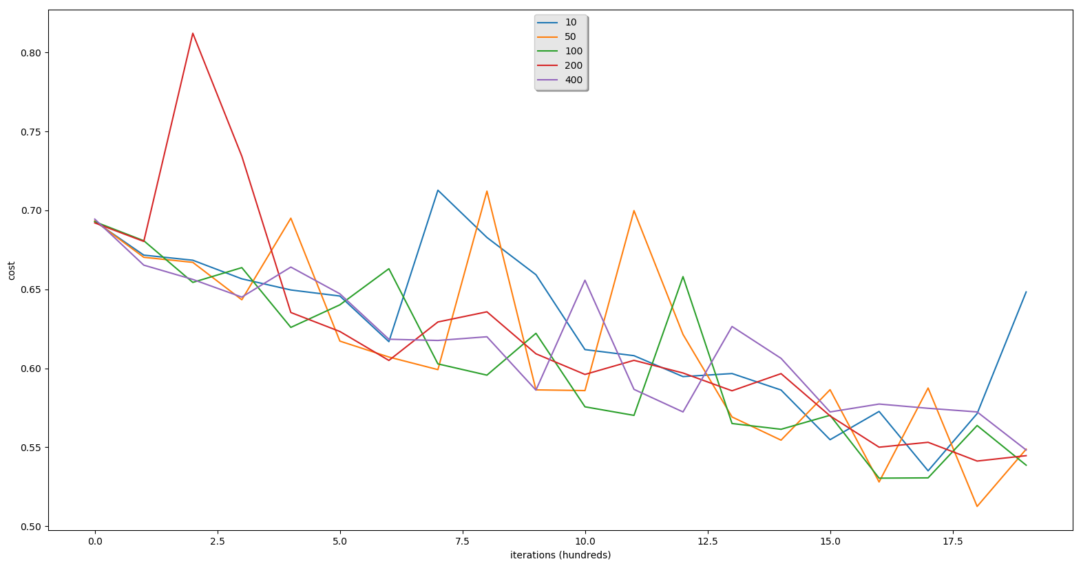
plt.show()

We'll receive such training and testing results with num_iterations = 2000 and learning_rate = 0.1:

hidden layer is: 10
Cost after iteration 1400: 0.586238
Cost after iteration 1600: 0.572674
Cost after iteration 1800: 0.571317
train accuracy: 74.20859713428857 %
test accuracy: 60.3 %
-------------------------------------------------------
hidden layer is: 50
Cost after iteration 1400: 0.554478
Cost after iteration 1600: 0.528002
Cost after iteration 1800: 0.512501
train accuracy: 70.37654115294902 %
test accuracy: 60.4 %
-------------------------------------------------------
hidden layer is: 100
Cost after iteration 1400: 0.561368
Cost after iteration 1600: 0.530406
Cost after iteration 1800: 0.563748
train accuracy: 70.35988003998668 %
test accuracy: 61.0 %
-------------------------------------------------------
hidden layer is: 200
Cost after iteration 1400: 0.596620
Cost after iteration 1600: 0.550028
Cost after iteration 1800: 0.541246
train accuracy: 69.86004665111629 %
test accuracy: 59.8 %
-------------------------------------------------------
hidden layer is: 400
Cost after iteration 1400: 0.606300
Cost after iteration 1600: 0.577356
Cost after iteration 1800: 0.572363
train accuracy: 71.242919026991 %
test accuracy: 60.4 %
-------------------------------------------------------

We'll receive such training and testing results with num_iterations = 10000 and learning_rate = 0.05:

hidden layer is: 10
Cost after iteration 9400: 0.296215
Cost after iteration 9600: 0.285913
Cost after iteration 9800: 0.440895
train accuracy: 82.3558813728757 %
test accuracy: 60.3 %
-------------------------------------------------------
hidden layer is: 50
Cost after iteration 9400: 0.126889
Cost after iteration 9600: 0.186118
Cost after iteration 9800: 0.138445
train accuracy: 94.65178273908697 %
test accuracy: 59.300000000000004 %
-------------------------------------------------------
hidden layer is: 100
Cost after iteration 9400: 0.161640
Cost after iteration 9600: 0.194643
Cost after iteration 9800: 0.105035
train accuracy: 79.35688103965344 %
test accuracy: 59.699999999999996 %
-------------------------------------------------------
hidden layer is: 200
Cost after iteration 9400: 0.113325
Cost after iteration 9600: 0.166675
Cost after iteration 9800: 0.133236
train accuracy: 89.4368543818727 %
test accuracy: 61.3 %
-------------------------------------------------------
hidden layer is: 400
Cost after iteration 9400: 3.607211
Cost after iteration 9600: 0.349736
Cost after iteration 9800: 0.157746
train accuracy: 97.3842052649117 %
test accuracy: 62.8 %
-------------------------------------------------------

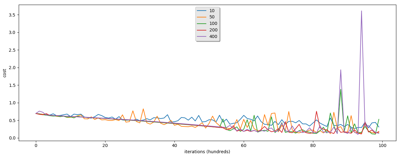
From these graphs, you can see that we are receiving much better train accuracy than testing. This is because of data overfitting. This means that it's quite hard for our model to predict animals with data it didn't saw before. We can't do anything better here with one hidden layer neural network. We'll see what we'll receive with a deep neural network.

By the way, you can see that our neural network with 400 hidden layers is just 3% better than our logistic regression model. It's not that impressive. We'll see what we can receive with the deeper network.

I uploaded the full tutorial code to the same GitHub page where I uploaded the logistic regression final code because we use the same dataset. After we finish our deep neural networks tutorial, we'll compare results from all of them.