Policy Optimization (PPO)

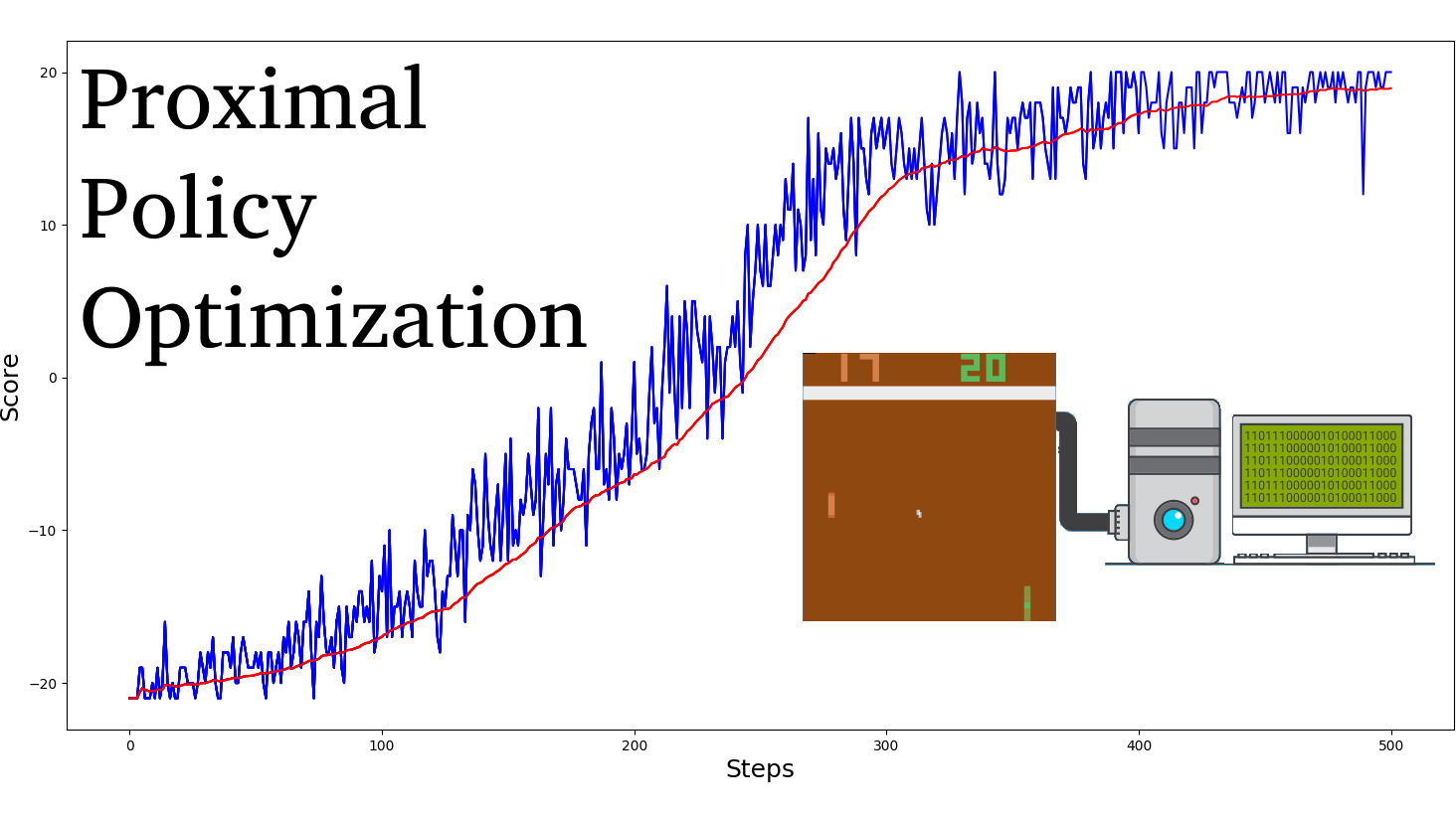
In 2018 OpenAI made a breakthrough in Deep Reinforcement Learning, this was possible only because of solid hardware architecture and using the state of the art's algorithm: Proximal Policy Optimization.

The main idea of Proximal Policy Optimization is to avoid having too large a policy update. To do that, we use a ratio that tells us the difference between our new and old policy and clip this ratio from 0.8 to 1.2. Doing that will ensure that the policy update will not be too large.

This tutorial will dive into understanding the PPO architecture and implement a Proximal Policy Optimization (PPO) agent that learns to play Pong-v0.

However, if you want to understand PPO, you need first to check all my previous tutorials. In this tutorial, as a backbone, I will use the A3C tutorial code.

Problem with Policy Gradient

If you were reading my tutorial about Policy Gradient, we talked about the Policy Loss function:

$L^{PG}\left(Q\right)=E_t\left[\log {\pi }_Q\left(a_t\right|s_t)\right]*A_t$

Here:

- L(Q) - Policy loss; E - Expected; logπ... - log probability of taking that action at that state, A - Advantage.

The idea of this function is doing gradient ascent step (which is equivalent to taking reversed gradient descent); this way, our agent is pushed to take actions that lead to higher rewards and avoid harmful actions.

However, the problem comes from the step size:

• Too small, the training process is too slow;
• Too high, there is too much variability in training.

That's where PPO is helpful; the idea is that PPO improves the stability of the Actor training by limiting the policy update at each training step.

To do that, PPO introduced a new objective function called "Clipped surrogate objective function" that will constrain policy change in a small range using a clip.

Clipped Surrogate Objective Function

First, as explained in the PPO paper, instead of using log pi to trace the impact of the actions, PPO uses the ratio between the probability of action under current policy divided by the likelihood of the action under the previous policy:

$r_t\left(Q\right)=\frac{{\pi }_Q\left(a_t\right|s_t)}{{\pi }_{Q_{old}}\left(a_t\right|s_t)}$

As we can see, r_t(Q) is the probability ratio between the new and old policy:

• If rt(Q) >1, the action is more probable in the current policy than the old one.
• If rt(Q) is between 0 and 1, the action is less likely for the current policy than for the old one.

As a consequence, we can write our new objective function:

$L^{CPI}\left(Q\right)={\hat{E}}_t\left[\frac{{\pi }_Q\left(a_t\right|s_t)}{{\pi }_{Q_{old}}\left(a_t\right|s_t)}{\hat{A}}_t\right]={\hat{E}}_t\left[r_t\left(Q\right){\hat{A}}_t\right]$

However, if the action took more probable in our current policy than in our former, this would lead to a giant policy gradient step and an excessive policy update.

Consequently, we need to constrain this objective function by penalizing changes that lead to a ratio (in the paper, it is said that the ratio can only vary from 0.8 to 1.2). To do that, we have to use the PPO clip probability ratio directly in the objective function with its Clipped surrogate objective function. By doing that, we'll ensure not to have too large policy update because the new policy can't be too different from the older one.

$L^{CLIP}\left(Q\right)={\hat{E}}_t\left[min\left(r_t\right(Q){\hat{A}}_t, clip(r_t\left(Q\right), 1-\in , 1+\in \left){\hat{A}}_t\right)\right]$

With the Clipped Surrogate Objective function, we have two probability ratios, one non-clipped and one clipped in a range (between [1−∈,1+∈], epsilon is a hyperparameter that helps us to define this clip range (in the paper ∈ = 0.2).

If we take the minimum of the clipped and non-clipped objectives, the final aim would be lower (pessimistic bound) than the unclipped goal. Consequently, we have two cases to consider:

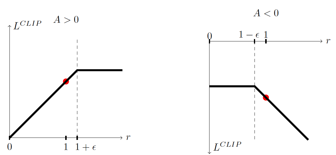
• When the advantage is > 0:

If advantage > 0, the action is better than the average of all the actions in that state. Therefore, we should encourage our new policy to increase the probability of taking that action at that state.

This means increasing r_t because we increase the probability at new policy and the denominator of old policy stay constant:

$L^{CPI}\left(Q\right)={\hat{E}}_t\left[\frac{{\pi }_Q\left(a_t\right|s_t)}{{\pi }_{Q_{old}}\left(a_t\right|s_t)}{\hat{A}}_t\right]={\hat{E}}_t\left[r_t\left(Q\right){\hat{A}}_t\right]$

However, because of the clip, rt(Q) will only grow to as much as 1+∈, which means this action can't be a hundred times probable compared to the old policy (because of the clip). This is done because we don't want to update our policy too much. Taking action at a specific state is only one try. It doesn't mean that it will always lead to a super positive reward, so we don't want to be too greedy because it can also lead to bad policy.

In summary, in the case of positive advantage, we want to increase the probability of taking that action at that step, but not too much.

• When the advantage is < 0:

If the advantage < 0, the action should be discouraged because of the negative effect of the outcome. Consequently, rt will decrease (because the action is less probable for the current agent policy than the previous one), but rt will only decrease to as little as 1−∈ because of the clip.

Also, we don't want to make a big change in the policy by being too greedy by ultimately reducing the probability of taking that action because it leads to an opposing advantage.

In summary, thanks to this clipped surrogate objective, the range that the new policy can vary from the old one is restricted because the incentive for the probability ratio to move outside of the interval is removed. If the ratio is > 1+e or < 1-e the gradient will be equal to 0 (no slope) because the clip has the effect to a gradient. So, both of these clipping regions do not allow us to become too greedy and try to upgrade too much at once and upgrade outside the region where this example is has a good approximation.

The final Clipped Surrogate Objective Loss:

$L_t^{CLIP+VF+S}\left(Q\right)={\hat{E}}_t\left[L_t^{CLIP}\left(Q\right)-c_1{L}^V{F}_t\left(Q\right)+c_{2}S\left[{\pi }_Q\right]\left(s_t\right)\right]$

Here:

- c1 and c2 - coefficients; S - denotes an entropy bonus, L^v and F_t - squared-error loss.

Implementing a PPO agent in A3C to play Pong:

So now, we're ready to implement a PPO agent in A3C style. This means that I will use A3C code as a backbone, and there will be the same processes explained in the A3C tutorial.

So, from the theory side, it looks that it's challenging to implement, but in practice, we already have prepared code to be adopted to use the PPO loss function; we will need to change our used loss function and defined replay function mainly:

def OurModel(input_shape, action_space, lr):
    X_input = Input(input_shape)

    X = Flatten(input_shape=input_shape)(X_input)

    X = Dense(512, activation="elu", kernel_initializer='he_uniform')(X)

    action = Dense(action_space, activation="softmax", kernel_initializer='he_uniform')(X)
    value = Dense(1, kernel_initializer='he_uniform')(X)

    def ppo_loss(y_true, y_pred):
        # Defined in https://arxiv.org/abs/1707.06347
        advantages, prediction_picks, actions = y_true[:, :1], y_true[:, 1:1+action_space], y_true[:, 1+action_space:]
        LOSS_CLIPPING = 0.2
        ENTROPY_LOSS = 5e-3

        prob = y_pred * actions
        old_prob = actions * prediction_picks
        r = prob/(old_prob + 1e-10)
        p1 = r * advantages
        p2 = K.clip(r, min_value=1 - LOSS_CLIPPING, max_value=1 + LOSS_CLIPPING) * advantages
        loss =  -K.mean(K.minimum(p1, p2) + ENTROPY_LOSS * -(prob * K.log(prob + 1e-10)))
        return loss

    Actor = Model(inputs = X_input, outputs = action)
    Actor.compile(loss=ppo_loss, optimizer=RMSprop(lr=lr))

    Critic = Model(inputs = X_input, outputs = value)
    Critic.compile(loss='mse', optimizer=RMSprop(lr=lr))

    return Actor, Critic

As you can see, we replace the categorical_crossentropy loss function with our ppo_loss function.

From the act function, we will need prediction:

def act(self, state):
    # Use the network to predict the next action to take, using the model
    prediction = self.Actor.predict(state)[0]
    action = np.random.choice(self.action_size, p=prediction)
    return action, prediction

Prediction from the above function is used in replay function:

def replay(self, states, actions, rewards, predictions):
    # reshape memory to appropriate shape for training
    states = np.vstack(states)
    actions = np.vstack(actions)
    predictions = np.vstack(predictions)

    # Compute discounted rewards
    discounted_r = np.vstack(self.discount_rewards(rewards))

    # Get Critic network predictions 
    values = self.Critic.predict(states)
    # Compute advantages
    advantages = discounted_r - values

    # stack everything to numpy array
    y_true = np.hstack([advantages, predictions, actions])
    
    # training Actor and Critic networks
    self.Actor.fit(states, y_true, epochs=self.EPOCHS, verbose=0, shuffle=True, batch_size=len(rewards))
    self.Critic.fit(states, discounted_r, epochs=self.EPOCHS, verbose=0, shuffle=True, batch_size=len(rewards))

You may ask, what is this np.hstack used for? Because we use a custom loss function, we must send data in the right shape of data. So we pack all advantages, predictions, actions to y_true, and when they are received in the custom loss function, we unpack them.

The last step to do is adding prediction memory to our run function:

def run(self):
    for e in range(self.EPISODES):
        state = self.reset(self.env)
        done, score, SAVING = False, 0, ''
        # Instantiate or reset games memory
        states, actions, rewards, predictions = [], [], [], []
        while not done:
            #self.env.render()
            # Actor picks an action
            action, prediction = self.act(state)
            # Retrieve new state, reward, and whether the state is terminal
            next_state, reward, done, _ = self.step(action, self.env, state)
            # Memorize (state, action, reward) for training
            states.append(state)
            action_onehot = np.zeros([self.action_size])
            action_onehot[action] = 1
            actions.append(action_onehot)
            rewards.append(reward)
            predictions.append(prediction)
            # Update current state
            state = next_state
            score += reward
            if done:
                average = self.PlotModel(score, e)
                # saving best models
                if average >= self.max_average:
                    self.max_average = average
                    self.save()
                    SAVING = "SAVING"
                else:
                    SAVING = ""
                print("episode: {}/{}, score: {}, average: {:.2f} {}".format(e, self.EPISODES, score, average, SAVING))

                self.replay(states, actions, rewards, predictions)
                
    self.env.close()

We add the same lines to the defined train_threading function. That's all! We have just created an agent that can learn to play any atari game. That's awesome! You'll need about 12 to 24 hours of training on 1 GPU to have a good agent with Pong-v0.

So this was a pretty long and exciting tutorial, and here is the complete code:

# Tutorial by www.pylessons.com
# Tutorial written for - Tensorflow 1.15, Keras 2.2.4

import os
import random
import gym
import pylab
import numpy as np
from keras.models import Model, load_model
from keras.layers import Input, Dense, Lambda, Add, Conv2D, Flatten
from keras.optimizers import Adam, RMSprop
from keras import backend as K
import cv2

import tensorflow as tf
from keras.backend.tensorflow_backend import set_session
import threading
from threading import Thread, Lock
import time

config = tf.ConfigProto()
config.gpu_options.allow_growth = True
sess = tf.Session(config=config)
set_session(sess)
K.set_session(sess)
graph = tf.get_default_graph()

def OurModel(input_shape, action_space, lr):
    X_input = Input(input_shape)

    #X = Conv2D(32, 8, strides=(4, 4),padding="valid", activation="elu", data_format="channels_first", input_shape=input_shape)(X_input)
    #X = Conv2D(64, 4, strides=(2, 2),padding="valid", activation="elu", data_format="channels_first")(X)
    #X = Conv2D(64, 3, strides=(1, 1),padding="valid", activation="elu", data_format="channels_first")(X)
    X = Flatten(input_shape=input_shape)(X_input)

    X = Dense(512, activation="elu", kernel_initializer='he_uniform')(X)
    #X = Dense(256, activation="elu", kernel_initializer='he_uniform')(X)
    #X = Dense(64, activation="elu", kernel_initializer='he_uniform')(X)

    action = Dense(action_space, activation="softmax", kernel_initializer='he_uniform')(X)
    value = Dense(1, activation='linear', kernel_initializer='he_uniform')(X)

    def ppo_loss(y_true, y_pred):
        # Defined in https://arxiv.org/abs/1707.06347
        advantages, prediction_picks, actions = y_true[:, :1], y_true[:, 1:1+action_space], y_true[:, 1+action_space:]
        LOSS_CLIPPING = 0.2
        ENTROPY_LOSS = 5e-3

        prob = y_pred * actions
        old_prob = actions * prediction_picks
        r = prob/(old_prob + 1e-10)
        p1 = r * advantages
        p2 = K.clip(r, min_value=1 - LOSS_CLIPPING, max_value=1 + LOSS_CLIPPING) * advantages
        loss =  -K.mean(K.minimum(p1, p2) + ENTROPY_LOSS * -(prob * K.log(prob + 1e-10)))
        return loss
        
    Actor = Model(inputs = X_input, outputs = action)
    Actor.compile(loss=ppo_loss, optimizer=RMSprop(lr=lr))

    Critic = Model(inputs = X_input, outputs = value)
    Critic.compile(loss='mse', optimizer=RMSprop(lr=lr))

    return Actor, Critic

class PPOAgent:
    # PPO Main Optimization Algorithm
    def __init__(self, env_name):
        # Initialization
        # Environment and PPO parameters
        self.env_name = env_name       
        self.env = gym.make(env_name)
        self.action_size = self.env.action_space.n
        self.EPISODES, self.episode, self.max_average = 10000, 0, -21.0 # specific for pong
        self.lock = Lock()
        self.lr = 0.0001

        self.ROWS = 80
        self.COLS = 80
        self.REM_STEP = 4
        self.EPOCHS = 10

        # Instantiate plot memory
        self.scores, self.episodes, self.average = [], [], []

        self.Save_Path = 'Models'
        self.state_size = (self.REM_STEP, self.ROWS, self.COLS)
        
        if not os.path.exists(self.Save_Path): os.makedirs(self.Save_Path)
        self.path = '{}_APPO_{}'.format(self.env_name, self.lr)
        self.Model_name = os.path.join(self.Save_Path, self.path)

        # Create Actor-Critic network model
        self.Actor, self.Critic = OurModel(input_shape=self.state_size, action_space = self.action_size, lr=self.lr)

        self.Actor._make_predict_function()
        self.Critic._make_predict_function()

        global graph
        graph = tf.get_default_graph()

    def act(self, state):
        # Use the network to predict the next action to take, using the model
        prediction = self.Actor.predict(state)[0]
        action = np.random.choice(self.action_size, p=prediction)
        return action, prediction

    def discount_rewards(self, reward):
        # Compute the gamma-discounted rewards over an episode
        gamma = 0.99    # discount rate
        running_add = 0
        discounted_r = np.zeros_like(reward)
        for i in reversed(range(0,len(reward))):
            if reward[i] != 0: # reset the sum, since this was a game boundary (pong specific!)
                running_add = 0
            running_add = running_add * gamma + reward[i]
            discounted_r[i] = running_add

        discounted_r -= np.mean(discounted_r) # normalizing the result
        discounted_r /= np.std(discounted_r) # divide by standard deviation
        return discounted_r

    def replay(self, states, actions, rewards, predictions):
        # reshape memory to appropriate shape for training
        states = np.vstack(states)
        actions = np.vstack(actions)
        predictions = np.vstack(predictions)

        # Compute discounted rewards
        discounted_r = np.vstack(self.discount_rewards(rewards))

        # Get Critic network predictions 
        values = self.Critic.predict(states)
        # Compute advantages
        advantages = discounted_r - values

        # stack everything to numpy array
        y_true = np.hstack([advantages, predictions, actions])
        
        # training Actor and Critic networks
        self.Actor.fit(states, y_true, epochs=self.EPOCHS, verbose=0, shuffle=True, batch_size=len(rewards))
        self.Critic.fit(states, discounted_r, epochs=self.EPOCHS, verbose=0, shuffle=True, batch_size=len(rewards))
 
    def load(self, Actor_name, Critic_name):
        self.Actor = load_model(Actor_name, compile=False)
        #self.Critic = load_model(Critic_name, compile=False)

    def save(self):
        self.Actor.save(self.Model_name + '_Actor.h5')
        #self.Critic.save(self.Model_name + '_Critic.h5')

    pylab.figure(figsize=(18, 9))
    def PlotModel(self, score, episode):
        self.scores.append(score)
        self.episodes.append(episode)
        self.average.append(sum(self.scores[-50:]) / len(self.scores[-50:]))
        if str(episode)[-2:] == "00":# much faster than episode % 100
            pylab.plot(self.episodes, self.scores, 'b')
            pylab.plot(self.episodes, self.average, 'r')
            pylab.ylabel('Score', fontsize=18)
            pylab.xlabel('Steps', fontsize=18)
            try:
                pylab.savefig(self.path+".png")
            except OSError:
                pass

        return self.average[-1]

    def imshow(self, image, rem_step=0):
        cv2.imshow(self.Model_name+str(rem_step), image[rem_step,...])
        if cv2.waitKey(25) & 0xFF == ord("q"):
            cv2.destroyAllWindows()
            return

    def GetImage(self, frame, image_memory):
        if image_memory.shape == (1,*self.state_size):
            image_memory = np.squeeze(image_memory)

        # croping frame to 80x80 size
        frame_cropped = frame[35:195:2, ::2,:]
        if frame_cropped.shape[0] != self.COLS or frame_cropped.shape[1] != self.ROWS:
            # OpenCV resize function 
            frame_cropped = cv2.resize(frame, (self.COLS, self.ROWS), interpolation=cv2.INTER_CUBIC)
        
        # converting to RGB (numpy way)
        frame_rgb = 0.299*frame_cropped[:,:,0] + 0.587*frame_cropped[:,:,1] + 0.114*frame_cropped[:,:,2]

        # convert everything to black and white (agent will train faster)
        frame_rgb[frame_rgb < 100] = 0
        frame_rgb[frame_rgb >= 100] = 255
        # converting to RGB (OpenCV way)
        #frame_rgb = cv2.cvtColor(frame_cropped, cv2.COLOR_RGB2GRAY)     

        # dividing by 255 we expresses value to 0-1 representation
        new_frame = np.array(frame_rgb).astype(np.float32) / 255.0

        # push our data by 1 frame, similar as deq() function work
        image_memory = np.roll(image_memory, 1, axis = 0)

        # inserting new frame to free space
        image_memory[0,:,:] = new_frame

        # show image frame   
        #self.imshow(image_memory,0)
        #self.imshow(image_memory,1)
        #self.imshow(image_memory,2)
        #self.imshow(image_memory,3)
        
        return np.expand_dims(image_memory, axis=0)

    def reset(self, env):
        image_memory = np.zeros(self.state_size)
        frame = env.reset()
        for i in range(self.REM_STEP):
            state = self.GetImage(frame, image_memory)
        return state

    def step(self, action, env, image_memory):
        next_state, reward, done, info = env.step(action)
        next_state = self.GetImage(next_state, image_memory)
        return next_state, reward, done, info
    
    def run(self):
        for e in range(self.EPISODES):
            state = self.reset(self.env)
            done, score, SAVING = False, 0, ''
            # Instantiate or reset games memory
            states, actions, rewards, predictions = [], [], [], []
            while not done:
                #self.env.render()
                # Actor picks an action
                action, prediction = self.act(state)
                # Retrieve new state, reward, and whether the state is terminal
                next_state, reward, done, _ = self.step(action, self.env, state)
                # Memorize (state, action, reward) for training
                states.append(state)
                action_onehot = np.zeros([self.action_size])
                action_onehot[action] = 1
                actions.append(action_onehot)
                rewards.append(reward)
                predictions.append(prediction)
                # Update current state
                state = next_state
                score += reward
                if done:
                    average = self.PlotModel(score, e)
                    # saving best models
                    if average >= self.max_average:
                        self.max_average = average
                        self.save()
                        SAVING = "SAVING"
                    else:
                        SAVING = ""
                    print("episode: {}/{}, score: {}, average: {:.2f} {}".format(e, self.EPISODES, score, average, SAVING))

                    self.replay(states, actions, rewards, predictions)
                    
        self.env.close()

    def train(self, n_threads):
        self.env.close()
        # Instantiate one environment per thread
        envs = [gym.make(self.env_name) for i in range(n_threads)]

        # Create threads
        threads = [threading.Thread(
                target=self.train_threading,
                daemon=True,
                args=(self,
                    envs[i],
                    i)) for i in range(n_threads)]

        for t in threads:
            time.sleep(2)
            t.start()

    def train_threading(self, agent, env, thread):
        global graph
        with graph.as_default():
            while self.episode < self.EPISODES:
                # Reset episode
                score, done, SAVING = 0, False, ''
                state = self.reset(env)
                # Instantiate or reset games memory
                states, actions, rewards, predictions = [], [], [], []
                while not done:
                    action, prediction = agent.act(state)
                    next_state, reward, done, _ = self.step(action, env, state)

                    states.append(state)
                    action_onehot = np.zeros([self.action_size])
                    action_onehot[action] = 1
                    actions.append(action_onehot)
                    rewards.append(reward)
                    predictions.append(prediction)
                    
                    score += reward
                    state = next_state

                self.lock.acquire()
                self.replay(states, actions, rewards, predictions)
                self.lock.release()

                # Update episode count
                with self.lock:
                    average = self.PlotModel(score, self.episode)
                    # saving best models
                    if average >= self.max_average:
                        self.max_average = average
                        self.save()
                        SAVING = "SAVING"
                    else:
                        SAVING = ""
                    print("episode: {}/{}, thread: {}, score: {}, average: {:.2f} {}".format(self.episode, self.EPISODES, thread, score, average, SAVING))
                    if(self.episode < self.EPISODES):
                        self.episode += 1
            env.close()            

    def test(self, Actor_name, Critic_name):
        self.load(Actor_name, Critic_name)
        for e in range(100):
            state = self.reset(self.env)
            done = False
            score = 0
            while not done:
                action = np.argmax(self.Actor.predict(state))
                state, reward, done, _ = self.step(action, self.env, state)
                score += reward
                if done:
                    print("episode: {}/{}, score: {}".format(e, self.EPISODES, score))
                    break
        self.env.close()

if __name__ == "__main__":
    #env_name = 'Pong-v0'
    agent = PPOAgent(env_name)
    #agent.run() # use as PPO
    agent.train(n_threads=5) # use as APPO
    #agent.test('Pong-v0_APPO_0.0001_Actor.h5', 'Pong-v0_APPO_0.0001_Critic.h5')

So same as before, I trained PongDeterministic-v4 and Pong-v0, from all my previous RL tutorials results, were the best. In PongDeterministic-v4, we reached the best score in around 400 steps (while A3C needed only 800 steps):

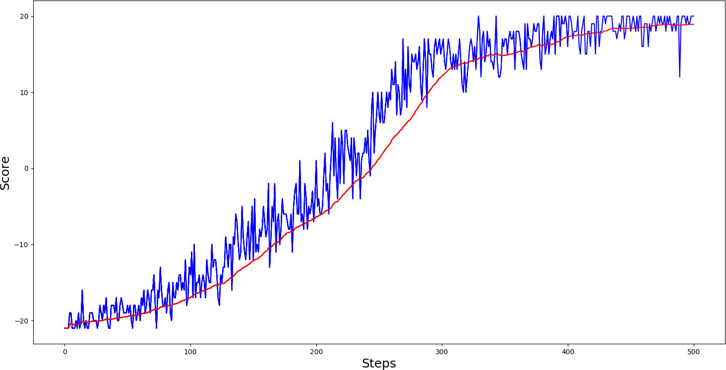
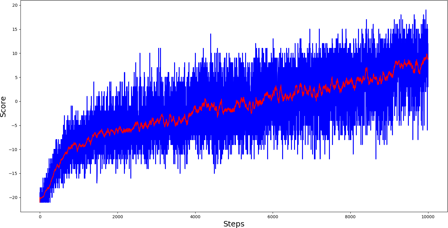
And here are the results for the Pong-v0 environment :

Results are pretty nice, comparing with other RL algorithms. I am delighted with the results! My goal wasn't to make it the best, to compare it with the same parameters.

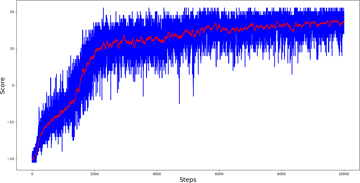
After training it, I thought that this algorithm should learn to play Pong with CNN layers, then my agent would be smaller, and I would be able to upload it to GitHub. So, I changed model architecture in the following way:

def OurModel(input_shape, action_space, lr):
    X_input = Input(input_shape)

    X = Conv2D(32, 8, strides=(4, 4),padding="valid", activation="elu", data_format="channels_first", input_shape=input_shape)(X_input)
    X = Conv2D(64, 4, strides=(2, 2),padding="valid", activation="elu", data_format="channels_first")(X)
    X = Conv2D(64, 3, strides=(1, 1),padding="valid", activation="elu", data_format="channels_first")(X)

    X = Dense(512, activation="elu", kernel_initializer='he_uniform')(X)

    action = Dense(action_space, activation="softmax", kernel_initializer='he_uniform')(X)
    value = Dense(1, kernel_initializer='he_uniform')(X)

    ...

And I was right! I trained this agent for 10k steps, and the results were also quite impressive:

Here is the gif, how my agent plays pong:

Conclusion:

Don't forget to implement each part of the code by yourself. It's essential to understand how everything works. Try to modify the hyperparameters, use another gym environment. Experimenting is the best way to learn, so have fun!

I hope this tutorial could give you a good idea of the basic PPO algorithm. You can now build upon this by executing multiple environments in parallel to collect more training samples and solve more complicated game scenarios.

For now, this is my last Reinforcement Learning tutorial. This was quite a long journey where I learned a lot. I plan to return to reinforcement learning later this year, and this will be a more practical and more exciting tutorial; we will use it in finance!