In this part, we will extend the code written in my previous tutorial to visualize the RL Bitcoin trading bot using Matplotlib and Python. If you haven't read my earlier tutorial and are not familiar with the code I wrote, I recommend reading it before reading this tutorial further.
If you are unfamiliar with the Matplotlib Python library, don't worry. I will be going over the code step-by-step, so you can create your custom visualization or modify mine according to your needs. If you can't understand everything, this tutorial code is always available on my GitHub repository.
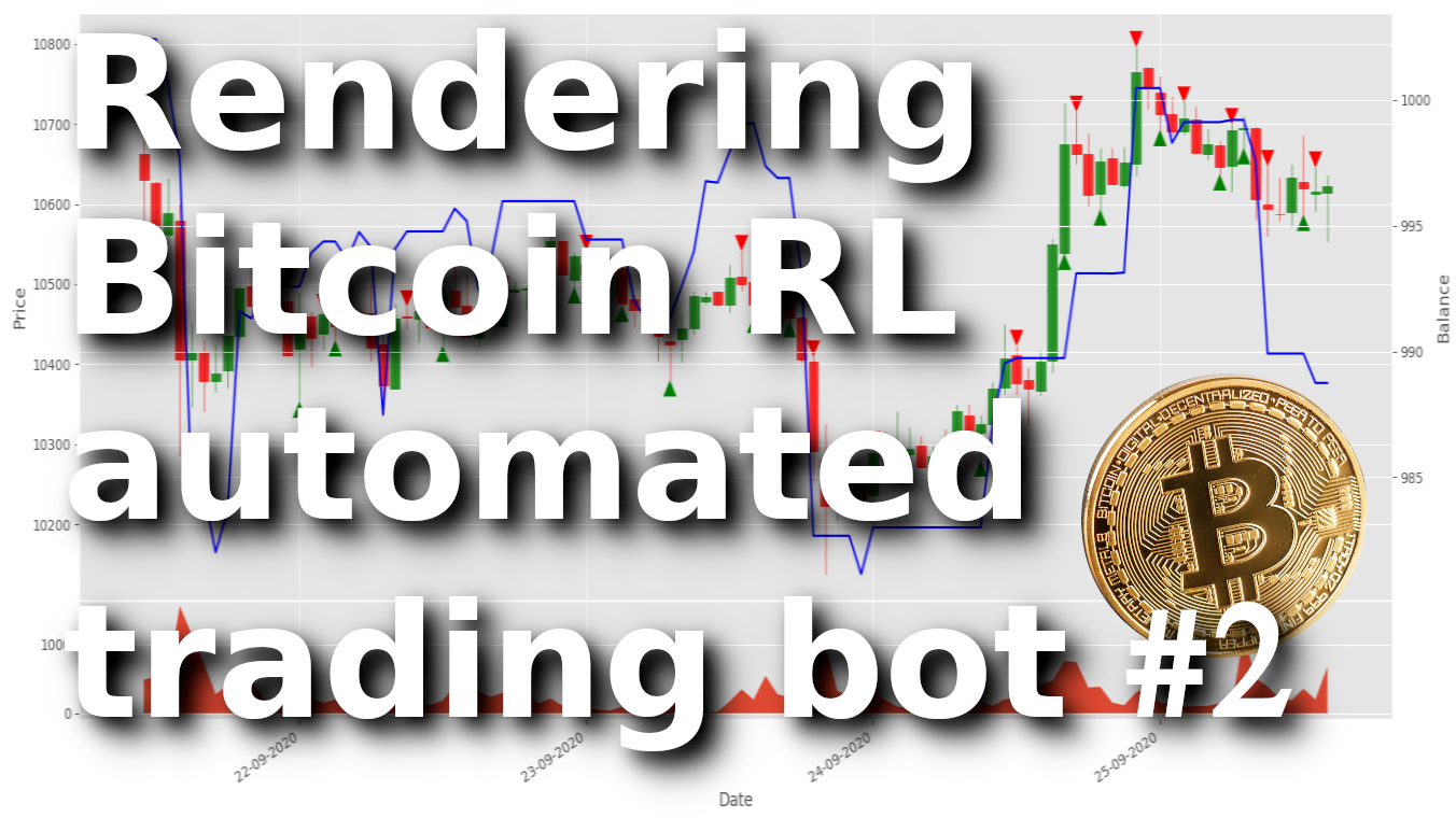
Before moving forward, I will show you a short preview of what we are going to create in this tutorial:
Let's begin! At first look, it might look quite complicated, but actually, it's not that hard. It's just a couple of parameters updating on each environment step with some essential information with the help of the Matplotlib already written functionality.
Bitcoin Trading bot Visualization
We wrote a simple render method using print statements to display the agent's net worth in our last tutorial. I could have added other essential metrics, but I left them to this tutorial. So, let's begin writing that logic to a new method file called utils.py to save a session's trading metrics to a file, if necessary. I'll start by creating a simple function called Write_to_file(), and we'll log everything that is sent to this function to a text file:
import os

def Write_to_file(Date, net_worth, filename='{}.txt'.format(datetime.now().strftime("%Y-%m-%d %H:%M:%S"))):
    for i in net_worth:
        Date += " {}".format(i)
    #print(Date)
    if not os.path.exists('logs'):
        os.makedirs('logs')
    file = open("logs/"+filename, 'a+')
    file.write(Date+"\n")
    file.close()
Now simply from our main code, I import it with from utils import Write_to_file. I prefer to call this function a step function, just after we do self.orders_history.append(..., I insert Write_to_file(Date, self.orders_history[-1]) code line, and it works. You can add more metrics to write to this file, but it was enough to find the first issue with my code.
I noticed that when my bot makes a buy operation, my balance is not zero, but is close to zero, more precisely -1.1368683772161603e-13. So instead of measuring if my balance is more than 0, I thought it would be better to measure if the current balance is more than 1% of my whole initial balance:
elif action == 1 and self.balance > self.initial_balance/100: But this tutorial is not about bugs and other improvements; let's move on to creating our new render method. It will utilize the new TradingGraph class that we haven't written yet; we'll get to that next. I am not going to show the full code here. I'll show you what's new on my code before using my TradingGraph:
class CustomEnv:
    def __init__(self, Render_range = 100):
        self.Render_range = Render_range # render range in visualization

    def reset(self):
        self.visualization = TradingGraph(Render_range=self.Render_range) # init visualization
        self.trades = deque(maxlen=self.Render_range) # limited orders memory for visualization

    def step(self, action):
        Date = self.df.loc[self.current_step, 'Date'] # for visualization
        High = self.df.loc[self.current_step, 'High'] # for visualization
        Low = self.df.loc[self.current_step, 'Low'] # for visualization

        if action == 0: # Hold
            pass
        elif action == 1 and self.balance > self.initial_balance/100:
            self.trades.append({'Date' : Date, 'High' : High, 'Low' : Low, 'total': self.crypto_bought, 'type': "buy"})
        elif action == 2 and self.crypto_held>0:
            self.trades.append({'Date' : Date, 'High' : High, 'Low' : Low, 'total': self.crypto_sold, 'type': "sell"})

        Write_to_file(Date, self.orders_history[-1])

    # render environment
    def render(self, visualize = False):
        #print(f'Step: {self.current_step}, Net Worth: {self.net_worth}')
        if visualize:
            Date = self.df.loc[self.current_step, 'Date']
            Open = self.df.loc[self.current_step, 'Open']
            Close = self.df.loc[self.current_step, 'Close']
            High = self.df.loc[self.current_step, 'High']
            Low = self.df.loc[self.current_step, 'Low']
            Volume = self.df.loc[self.current_step, 'Volume']

            # Render the environment to the screen
            self.visualization.render(Date, Open, High, Low, Close, Volume, self.net_worth, self.trades)
Here, above, is the main changes from my previous tutorial part. As you can see, in the __init__ part, we must initialize our render range. This means how many bars of history we would like to render.
In the reset function, we create a new object with our TradingGraph class. And of course, we make a limited size deque of trades list. We'll use this list to put all orders (buy/sell) that our bot does so that we can draw them on our beautiful plot.
In the step function, we get the main points of our price (date, high, Low), and when our bot does some order, we'll put this information to our trades list as a dictionary.
And the last modified function is a render. As you can see, we can turn on/off visualization with the True/False parameters. Here we take all necessary (Date, Open, Close, High, Low, Volume) parameters and call self.visualization.render function. Also, because we want to show how our net worth changes and where our bot makes sell or buy orders, we'll send self.net_worth and self.trades parameters to the same function.
Now our TradingGraph has all of the information it needs to render the market price history and trade volume, along with our agent's net worth and any trades it's made. Let's get started rendering our visualization! First, we'll import all necessary libraries for our graph, then we'll define our TradingGraph, and its __init__ method. Here is where we will create our matplotlib figure and set up each subplot to be rendered.
Here I create the first look of our chart by defining style and figure size. First, we define some deque lists, where we'll save our temporary information for our graph. Also, I am closing all plots in case there are open — this is necessary when we want to start rendering the second episode graph (agent resets and reinitializes every episode).
import pandas as pd
from collections import deque
import matplotlib.pyplot as plt
from mplfinance.original_flavor import candlestick_ohlc
import matplotlib.dates as mpl_dates
from datetime import datetime
import os
import cv2
import numpy as np

class TradingGraph:
    # A crypto trading visualization using matplotlib made to render custom prices which come in following way:
    # Date, Open, High, Low, Close, Volume, net_worth, trades
    # call render every step
    def __init__(self, Render_range):
        self.Volume = deque(maxlen=Render_range)
        self.net_worth = deque(maxlen=Render_range)
        self.render_data = deque(maxlen=Render_range)
        self.Render_range = Render_range

        # We are using the style ‘ggplot’
        plt.style.use('ggplot')
        # close all plots if there are open
        plt.close('all')
        # figsize attribute allows us to specify the width and height of a figure in unit inches
        self.fig = plt.figure(figsize=(16,8))

        # Create top subplot for price axis
        self.ax1 = plt.subplot2grid((6,1), (0,0), rowspan=5, colspan=1)

        # Create bottom subplot for volume which shares its x-axis
        self.ax2 = plt.subplot2grid((6,1), (5,0), rowspan=1, colspan=1, sharex=self.ax1)

        # Create a new axis for net worth which shares its x-axis with price
        self.ax3 = self.ax1.twinx()

        # Formatting Date
        self.date_format = mpl_dates.DateFormatter('%d-%m-%Y')
        #self.date_format = mpl_dates.DateFormatter('%d-%m-%Y')

        # Add paddings to make graph easier to view
        #plt.subplots_adjust(left=0.07, bottom=-0.1, right=0.93, top=0.97, wspace=0, hspace=0)

        # we need to set layers
        self.ax2.set_xlabel('Date')
        self.ax1.set_ylabel('Price')
        self.ax3.set_ylabel('Balance')

        # I use tight_layout to replace plt.subplots_adjust
        self.fig.tight_layout()

        # Show the graph with matplotlib
        plt.show()
As you can see, we use the plt.subplot2grid(...) method to first create a main subplot at the top of our figure to render our market candlestick data, and then we make another subplot below it for our volume. And last, we create a third axis, with twinx() function, which allows us to overlay another grid on top that will share the same x-axis. The first argument of the subplot2grid function is the size of the subplot and the second is the location within the figure.
Usually, we plot some graphs with the matplotlib library. Mostly there are large white margins, which makes our graph smaller, so it's recommended to remove them. Until now, I used subplot_adjust() function, but I found that tigh_layout() is much better; we don't need to measure our white margin sizes. Also, it's unnecessary, but our chart with labels on sides looks much better, so I set the Date, Price, Balance axis not to forget to do that in the future. Finally, and most importantly, we will render our figure to the screen using plt.show():
Next, let's write our render method. This will take all the information from the current time step and render a live representation to the screen. One of the most complicated things is rendering a price graph. But luckily, to keep things simple, we can use OHCL bars from the mplfinance library we imported before. If you don't already have it, write pip install mplfinance, as this package is the easiest way for the candlestick graphs to be plotted.
The date2num function is used to reformat dates into timestamps, necessary in the OHCL rendering process. Every render step we append our necessary OHCL data to deque memory, which is rendered on our plot. Because our graph is dynamic, we must clear the previous frame before generating a new one. After doing so, we take the OHCL data and render a candlestick graph to the self.ax1 subplot.
Because we are clearing our all axis every frame, our labels are also cleared, so we move them from __init__ part to render part. Finally, and most importantly, we will render our figure to the screen using plt.show(block=False). If you forget to pass block=False, you will only ever see the first step rendered, after which the agent will be blocked from continuing. It's essential to call plt.pause(); otherwise, each frame will be cleared by the next call to render before the last frame was actually shown on screen.
class TradingGraph:
    def __init__(self, Render_range):
        ...

    # Render the environment to the screen
    def render(self, Date, Open, High, Low, Close, Volume, net_worth, trades):
        # before appending to deque list, need to convert Date to special format
        Date = mpl_dates.date2num([pd.to_datetime(Date)])[0]
        self.render_data.append([Date, Open, High, Low, Close])

        # Clear the frame rendered last step
        self.ax1.clear()
        candlestick_ohlc(self.ax1, self.render_data, width=0.8/24, colorup='green', colordown='red', alpha=0.8)

        # we need to set layers every step, because we are clearing subplots every step
        self.ax2.set_xlabel('Date')
        self.ax1.set_ylabel('Price')
        self.ax3.set_ylabel('Balance')

        """Display image with matplotlib - interrupting other tasks"""
        # Show the graph without blocking the rest of the program
        plt.show(block=False)
        # Necessary to view frames before they are unrendered
        plt.pause(0.001)
After implementing the above code, we should see beautiful OHCL bars on our screen:
So, the hardest part was done already; now we would like to add Volume and Net Worth and beautifully formated Dates to our plot. The same as we did with our OHCL data, we should collect volume and net worth history data by appending them to the deque list. Similarly, we clear ax2 and ax3 subplots, put all dates to one list, and fill the ax2 subplot with our historical volumes. The most important lines are self.ax1.xaxis.set_major_formatter(self.date_format) and self.fig.autofmt_xdate(), where all the beautiful date formatting is done. To add net worth is one of the simplest parts, we add the following line self.ax3.plot(Date_Render_range, self.net_worth, color=”blue”). Here is the code up to this point:
class TradingGraph:
    def __init__(self, Render_range):
        ...

    # Render the environment to the screen
    def render(self, Date, Open, High, Low, Close, Volume, net_worth, trades):
        # append volume and net_worth to deque list
        self.Volume.append(Volume)
        self.net_worth.append(net_worth)

        # before appending to deque list, need to convert Date to special format
        Date = mpl_dates.date2num([pd.to_datetime(Date)])[0]
        self.render_data.append([Date, Open, High, Low, Close])

        # Clear the frame rendered last step
        self.ax1.clear()
        candlestick_ohlc(self.ax1, self.render_data, width=0.8/24, colorup='green', colordown='red', alpha=0.8)

        # Put all dates to one list and fill ax2 sublot with volume
        Date_Render_range = [i[0] for i in self.render_data]
        self.ax2.clear()
        self.ax2.fill_between(Date_Render_range, self.Volume, 0)

        # draw our net_worth graph on ax3 (shared with ax1) subplot
        self.ax3.clear()
        self.ax3.plot(Date_Render_range, self.net_worth, color="blue")

        # beautify the x-labels (Our Date format)
        self.ax1.xaxis.set_major_formatter(self.date_format)
        self.fig.autofmt_xdate()

        # we need to set layers every step, because we are clearing subplots every step
        self.ax2.set_xlabel('Date')
        self.ax1.set_ylabel('Price')
        self.ax3.set_ylabel('Balance')

        # I use tight_layout to replace plt.subplots_adjust
        self.fig.tight_layout()

        """Display image with matplotlib - interrupting other tasks"""
        # Show the graph without blocking the rest of the program
        plt.show(block=False)
        # Necessary to view frames before they are unrendered
        plt.pause(0.001)
As you can see, now our chart is quite informative, there are many ways to improve it, but at this point, we mostly would like to know where our orders were made, so we need to add some arrow points.
To find how to add beautiful red and green arrows to our plot took me a while. But finally, I found the commonly used plot type "scatter plot", a close cousin of the line plot. Instead of points being joined by line segments, the points are represented individually with a dot, circle, or other shapes. This is the place where we'll use our self.trades dictionary from our main program. This place might be a little slower because I am using for loop to find date position, where our orders were made in plot history. I put a green or red arrow according to the order type, now the code looks quite simple, but I think this part took me the most time.
class TradingGraph:
    def __init__(self, Render_range):
        ...

    # Render the environment to the screen
    def render(self, Date, Open, High, Low, Close, Volume, net_worth, trades):
        # append volume and net_worth to deque list
        self.Volume.append(Volume)
        self.net_worth.append(net_worth)

        # before appending to deque list, need to convert Date to special format
        Date = mpl_dates.date2num([pd.to_datetime(Date)])[0]
        self.render_data.append([Date, Open, High, Low, Close])

        # Clear the frame rendered last step
        self.ax1.clear()
        candlestick_ohlc(self.ax1, self.render_data, width=0.8/24, colorup='green', colordown='red', alpha=0.8)

        # Put all dates to one list and fill ax2 sublot with volume
        Date_Render_range = [i[0] for i in self.render_data]
        self.ax2.clear()
        self.ax2.fill_between(Date_Render_range, self.Volume, 0)

        # draw our net_worth graph on ax3 (shared with ax1) subplot
        self.ax3.clear()
        self.ax3.plot(Date_Render_range, self.net_worth, color="blue")

        # beautify the x-labels (Our Date format)
        self.ax1.xaxis.set_major_formatter(self.date_format)
        self.fig.autofmt_xdate()

        # sort sell and buy orders, put arrows in appropiate order positions
        for trade in trades:
            trade_date = mpl_dates.date2num([pd.to_datetime(trade['Date'])])[0]
            if trade_date in Date_Render_range:
                if trade['type'] == 'buy':
                    high_low = trade['Low']-10
                    self.ax1.scatter(trade_date, high_low, c='green', label='green', s = 120, edgecolors='none', marker="^")
                else:
                    high_low = trade['High']+10
                    self.ax1.scatter(trade_date, high_low, c='red', label='red', s = 120, edgecolors='none', marker="v")

        # we need to set layers every step, because we are clearing subplots every step
        self.ax2.set_xlabel('Date')
        self.ax1.set_ylabel('Price')
        self.ax3.set_ylabel('Balance')

        # I use tight_layout to replace plt.subplots_adjust
        self.fig.tight_layout()

        """Display image with matplotlib - interrupting other tasks"""
        # Show the graph without blocking the rest of the program
        #plt.show(block=False)
        # Necessary to view frames before they are unrendered
        #plt.pause(0.001)

        """Display image with OpenCV - no interruption"""
        # redraw the canvas
        self.fig.canvas.draw()
        # convert canvas to image
        img = np.fromstring(self.fig.canvas.tostring_rgb(), dtype=np.uint8, sep='')
        img  = img.reshape(self.fig.canvas.get_width_height()[::-1] + (3,))

        # img is rgb, convert to opencv's default bgr
        image = cv2.cvtColor(img, cv2.COLOR_RGB2BGR)

        # display image with OpenCV or any operation you like
        cv2.imshow("Bitcoin trading bot",image)

        if cv2.waitKey(25) & 0xFF == ord("q"):
            cv2.destroyAllWindows()
            return
Also, you might see that I commended plt.show(block=False) function; instead, I wrote cv2 functions to show our image. I did this because while using matplotlib visualization every step, all our tasks were interrupted. We can't continue to write code, minimize it, or do any typing with our keyboard. As a workaround, I found that the best solution is to use the OpenCV library. And here is the final beautiful visualization of our Bitcoin trading BOT making actions.
Conclusion:
And that's it! We now have a beautiful, live rendering visualization of the random Bitcoin trading environment we created in the previous tutorial! We still haven't put much time into teaching the agent how to make money… We'll do that in the next tutorial!
We did a tremendous job here, and now when we have our trained agent doing some specific actions, we'll be able to evaluate if these actions were better than random or they weren't.
Thanks for reading! See you in the next part, where we'll add some neurons to our agent's brain! As always, all the code given in this tutorial can be found on my GitHub page and is free to use!