Deep Learning Introduction to TensorFlow

Welcome to the second tutorial. Until now, we have used NumPy to build neural networks. Now I will step you through a deep learning framework that will allow you to build neural networks more easily. Machine learning frameworks like TensorFlow can speed up your machine learning development significantly. These frameworks have a lot of documentation, which you should feel free to read. In this tutorial, I will teach to do the following in TensorFlow:

• Initialize variables;
• Start your own session.

Programing frameworks can not only shorten our coding time but sometimes also perform optimizations that speed up our coding.

1 - Exploring Tensorflow basics:

Let's begin with imports:

import os
os.environ['CUDA_VISIBLE_DEVICES'] = '-1'
import numpy as np
import tensorflow as tf

We will start with an example, where I'll compute for you the loss of one training example:

$loss=L(\hat{y}, y)={({\hat{y}}^{\left(i\right)}-y^{\left(i\right)})}^2$

# Define y_hat constant. Set to 36.
y_hat = tf.constant(36, name='y_hat')
# Define y. Set to 39
y = tf.constant(39, name='y')

# Create a variable for the loss
loss = tf.Variable((y - y_hat)**2, name='loss')

# When init is run later (session.run(init)),
# the loss variable will be initialized and ready to be computed
init = tf.global_variables_initializer()         

# Create a session and print the output
with tf.Session() as session:
	# Initializes the variables                    
    session.run(init)
    # Prints the loss                            
    print(session.run(loss))

Output:

9

Writing and running programs in TensorFlow has the following steps:

1. Create Tensors (variables) that are not yet executed/evaluated;
2. Write operations between those Tensors;
3. Initialize your Tensors;
4. Create a Session;
5. Run the Session. This will run the operations you'd written above.

Therefore, when we created a variable for the loss, we defined the loss as a function of other quantities but did not evaluate its value. To evaluate it, we had to run init=tf.global_variables_initializer(). This line initialized the loss variable, and in the last line, we were finally able to evaluate the value of loss and print its value.

Now let's look at an easy example. Run the cell below:

a = tf.constant(5)
b = tf.constant(10)
c = tf.multiply(a,b)
print(c)

Output:

Tensor("Mul_4:0", shape=(), dtype=int32)

As expected, you will not see 50! You got a tensor saying that the result is a tensor that does not have the shape attribute and type "int32". All you did was put in the 'computation graph', but you have not run this computation yet. To actually multiply the two numbers, you will have to create a session and run it:

sess = tf.Session()
print(sess.run(c))

Output:

50

Great! To summarize, remember to initialize your variables, create a session and run the operations inside the session.

Next, we also have to know about placeholders. A placeholder is an object whose value you can specify only later. To specify values for a placeholder, you can pass in values using a "feed dictionary" (feed_dict variable). Below, I created a placeholder for x. This allows us to pass in a number later when we run the session.

# Change the value of x in the feed_dict

x = tf.placeholder(tf.int64, name = 'x')
print(sess.run(2 * x, feed_dict = {x: 3}))
sess.close()

Output:

6

When we first defined x, we didn't have to specify a value for it. A placeholder is simply a variable that you will assign data to only later when running the session. We say that you feed data to these placeholders when running the session.

Here's what's happening: When you specify the operations needed for computation, you tell TensorFlow how to construct a computation graph. The computation graph can have some placeholders whose values you will specify only later. Finally, when you run the session, you are telling TensorFlow to execute the computation graph.

1.1 - Linear function:

Let's compute the following equation: Y=WX+b, where W and X are random matrices and b is a random vector.

W is of shape (4, 3), X is (3,1), and b is (4,1).

def linear_function():   
    # Initializes W to be a random tensor of shape (4,3)
    X = tf.constant(np.random.randn(3,1), name = "X")
    # Initializes X to be a random tensor of shape (3,1)
    W = tf.constant(np.random.randn(4,3), name = "W")
    # Initializes b to be a random tensor of shape (4,1)
    b = tf.constant(np.random.randn(4,1), name = "b")
    # Y = WX + b 
    Y = tf.add(tf.matmul(W,X),b)
    
    # Create the session using tf.Session() and run it with sess.run(...) on the variable we want to calculate  
    sess = tf.Session()
    result = sess.run(Y)
    
    # close the session 
    sess.close()

    return result

print( "result = ",linear_function())

Output:

result =  [[ 3.30652566]
 [ 0.43876476]
 [-3.14835357]
 [ 2.29081716]]

1.2 - Computing the sigmoid:

We just implemented a linear function. Tensorflow offers a variety of commonly used neural network functions like tf.sigmoid and tf.softmax. For this exercise, let's compute the sigmoid function of the input.

We will do this using a placeholder variable x. When running the session, we should use the feed dictionary to pass in the input z. So, we will have to:
1. create a placeholder x;
2. define the operations needed to compute the sigmoid using tf.sigmoid, and then;
3. run the session.

Note that there are two typical ways to create and use sessions in TensorFlow:

Method 1:

sess = tf.Session()
# Run the variables initialization (if needed), run the operations
result = sess.run(..., feed_dict = {...})
sess.close() # Close the session

Method 2:

with tf.Session() as sess: 
    # run the variables initialization (if needed), run the operations
    result = sess.run(..., feed_dict = {...})
    # This takes care of closing the session for you :)

Now we'll use 2nd method:

def sigmoid(z):   
    # Create a placeholder for x. Name it 'x'.
    x = tf.placeholder(tf.float32, name = 'x')

    # compute sigmoid(x)
    sigmoid = tf.sigmoid(x)

    # Create a session, and run it. 
    # We should use a feed_dict to pass z's value to x. 
    with tf.Session() as sess:
        # Run session and call the output "result"
        result = sess.run(sigmoid, feed_dict = {x: z})
    
    return result

print("sigmoid(0) = " + str(sigmoid(0)))
print("sigmoid(12) = " + str(sigmoid(12)))

Output:

sigmoid(0) = 0.5
sigmoid(12) = 0.9999938

To summarize, now we know how to:
1. Create placeholders;
2. Specify the computation graph corresponding to operations you want to compute;
3. Create the session;
4. Run the session and using a feed dictionary to specify placeholder variable values.

1.3 - Computing the cost:

We can also use a built-in function to compute the cost of our neural network. So instead of needing to write code to compute this as a function of a and y for i=1...m:

$J=-\frac{1}{m}\sum _{i=1}^m\left(y^{\left(i\right)}\log \left(a^{\left[2\right]\left(i\right)}\right)+(1-y^{\left(i\right)})\log (1-a^{\left[2\right]\left(i\right)})\right)$

We can do it in one line of code in TensorFlow!

The function we will use is:
tf.nn.sigmoid_cross_entropy_with_logits(logits = ..., labels = ...)

Our code should input z, compute the sigmoid (to get a), and then compute the cross-entropy cost J. All this can be done using one call to tf.nn.sigmoid_cross_entropy_with_logits, which computes the above-given cost formula of J:

def cost(logits, labels):     
    # Create the placeholders for "logits" (z) and "labels" (y)
    z = tf.placeholder(tf.float32, name = 'z')
    y = tf.placeholder(tf.float32, name = 'y')
    
    # Use the loss function
    cost = tf.nn.sigmoid_cross_entropy_with_logits(logits = z, labels = y)
    
    # Create a session (method 1 above)
    sess = tf.Session()
    
    # Run the session
    cost = sess.run(cost, feed_dict = {z: logits, y: labels})
    
    # Close the session (method 1 above)
    sess.close()
    
    return cost

logits = sigmoid(np.array([0.2,0.4,0.7,0.9]))
cost = cost(logits, np.array([0,0,1,1]))
print ("cost = ", cost)

Output:

cost = [1.0053872 1.0366408 0.41385433 0.39956617]

1.4 - Using One Hot encoding:

In deep learning, we will have a y vector with numbers ranging from 0 to C-1, where C is the number of classes. If C is, for example, 4, then you might have the following y vector, which you will need to convert as follows:

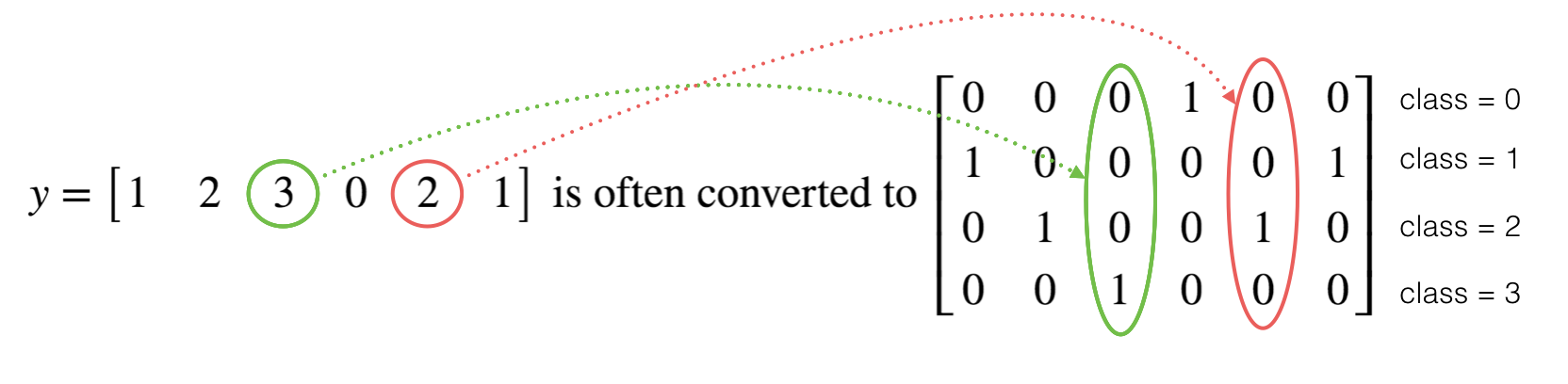
This is called a "one-hot" encoding because, in the converted representation, exactly one element of each column is "hot" (meaning set to 1). To do this conversion in NumPy, you might have to write a few lines of code. In TensorFlow, we can use one line of code:

tf.one_hot(labels, depth, axis)

We'll implement the function below to take one vector of labels and the total number of classes 𝐶 and return the one-hot encoding.

def one_hot_matrix(labels, C):
        
    # Create a tf.constant equal to C (depth), with name 'C'.
    C = tf.constant(C, name = "C")
    
    # Use tf.one_hot, be careful with the axis
    one_hot_matrix = tf.one_hot(labels, C, axis=0)
    
    # Create the session
    sess = tf.Session()
    
    # Run the session
    one_hot = sess.run(one_hot_matrix)
    
    # Close the session (method 1 above)
    sess.close()
    
    return one_hot

labels = np.array([1,2,3,0,2,1])
one_hot = one_hot_matrix(labels, C = 4)
print ("one_hot = ")
print (one_hot)

Output:

one_hot = 
[[0. 0. 0. 1. 0. 0.]
 [1. 0. 0. 0. 0. 1.]
 [0. 1. 0. 0. 1. 0.]
 [0. 0. 1. 0. 0. 0.]]

1.5 - Initialize with zeros and ones:

Now we will learn how to initialize a vector of zeros and ones. The function we will be calling is tf.ones(). To initialize with zeros, we could use tf.zeros() instead. These functions take in shape and return an array of dimension shape full of zeros and ones, respectively.

def ones(shape):
    # Create "ones" tensor using tf.ones(...).
    ones = tf.ones(shape)
    
    # Create the session
    sess = tf.Session()
    
    # Run the session to compute 'ones'
    ones = sess.run(ones)
    
    # Close the session (method 1 above)
    sess.close()
    
    return ones

print("ones = ")
print(ones((5,3)))

Output:

ones = 
[[1. 1. 1.]
 [1. 1. 1.]
 [1. 1. 1.]
 [1. 1. 1.]
 [1. 1. 1.]]

Conclusion: