Probably we all understand that computers and algorithms are getting better every day at "thinking", analyzing situations, and making decisions similar to humans do. Understanding computer vision is an integral part of this progress in the area of machine intelligence. Ten years ago, object detection was a mystery; it was not even worth mentioning object tracking. These technologies have come far in that regard, and the boundaries are being challenged and pushed as we talk.

While object detection in the image is receiving a lot of attention from the scientific community, a lesser-known area with widespread applications is object tracking in video or real-time video streaming. That's something that requires us to merge our knowledge of detecting objects in images with analyzing temporal information and using it to predict movement trajectories.

Object tracking might be used in sports events, for example, tracking basketball, catching burglars, counting passing cars in the street, or even tracking when your dog is running outside the house. There are many areas where we can use object tracking.

Object detection vs. Object Tracking

If you are new to computer vision and deep learning, you may ask, what's the difference between "Object Detection" and "Object Tracking"?

In simple terms, in object detection, we detect an object in a frame, put a bounding box or a mask around it, and classify the object. Note that the job of the detector ends here. It processes each frame independently and identifies numerous objects in that particular frame.

Now, an object tracker, on the other hand, needs to track a particular object across the entire series of frames (for example, video). If the detector detects two bananas in the frame, the object tracker has to identify the two separate detections and track them across the subsequent frames (with the help of a unique object ID).

Challenges

Tracking an object on a straight road or a clear area might sound very easy. But hardly any real-world application is that straightforward and free of any challenges. Here I will mention some common problems that might encounter while using an object tracker.

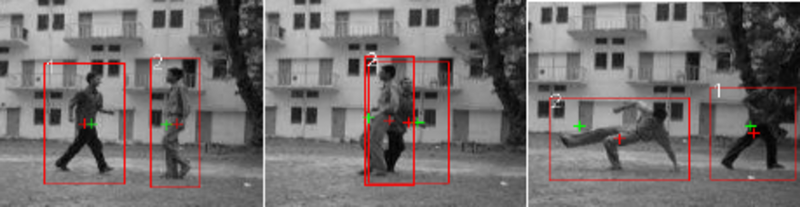
Occlusion:

The occlusion of objects in videos is one of the most common obstacles to the seamless tracking of objects. As you can see, in the above figure (left), the man in the background is detected, while the same guy goes undetected in the next frame (right). Now, the challenge for the tracker lies in identifying the same guy when he is detected in a much later frame and associating his older track and features with his trajectory.

In real-life examples, the task would be to track an object across different cameras, this may be used in AI stores where there is no cashier, and we must track a customer throughout the store. A similar example is illustrated above, as a consequence of this, there will be significant changes in how we view the object in each camera. In such cases, the features used to track an object become very important as we need to make sure they are invariant to the changes in views.

Non-stationary camera:

When the camera used for tracking a particular object is also in motion, it can often lead to unintended consequences. As I mentioned previously, many trackers consider the features from an object to track them. Such a tracker might fail in scenarios where the object appears different because of the camera motion (appear bigger or smaller). A robust tracker for this problem can be beneficial in critical applications like object tracking drones or autonomous navigation.

Annotating training data:

One of the most annoying things about building an object tracker is getting good training data for a particular scenario. Unlike building a dataset for an object detector, we can have randomly unconnected images. In object tracking, it's required to have video or frame sequences where each instance of the object is uniquely identified for each frame.

Traditional Methods

Mean shift method:

Mean-shift or "Mode seeking" is a popular algorithm mainly used in clustering and other related unsupervised problems. It is similar to K-Means but replaces the simple centroid technique of calculating the cluster centers with a weighted average that emphasizes points closer to the mean. The goal of the algorithm is to find all the modes in the provided data distribution. Also, this algorithm does not require an optimum "K" value like K-Means.

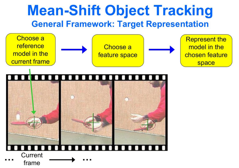
Suppose we detect an object in the frame and extract specific features from the detection (color, texture, histogram, etc.). By applying the mean-shift algorithm, we have a general idea of where the mode of the distribution of features lies in the current state. When we have the next frame, where this distribution has changed due to the object's movement in the frame, the mean-shift algorithm looks for the new largest mode and tracks the object.

For more info on the mean shift, refer to here.

Optical flow method:

This method differs from mean-shift, as we do not necessarily use features extracted from the detected object. Instead, the object is tracked using the Spatio-temporal image brightness variations at a pixel level.

Here we focus on obtaining a displacement vector for the object to be tracked across the frames. Tracking with optical flow rests on four essential assumptions:

1. Brightness consistency: Brightness around a small region is assumed to remain nearly constant, although the location of the area might change;
2. Spatial coherence: Neighboring points in the scene typically belong to the same surface and hence usually have similar motions;
3. Temporal persistence: Motion of a patch has a gradual change;
4. Limited motion: Points do not move very far or randomly.

Once these criteria are satisfied, we use the Lucas-Kanade method to obtain an equation for the velocity of specific points to be tracked (there are easily detected features usually). Using the equation and some prediction techniques, a given object can be tracked throughout the video frames.

For more info on Optical flow, refer to here.

Kalman Filter

In almost any engineering problem that involves prediction in a temporal or time series sense, it can be computer vision, guidance, navigation, stabilizing systems, or even economics; you may often hear "Kalman Filter".

The core idea of a Kalman filter is to use the available detections and previous predictions to arrive at the best guess of the current state while keeping the possibility of errors in the process.

For example, now we can train a fairly good YOLOv3 object detector that detects a person. But it is not that accurate and occasionally misses detections, say 10% of frames. To effectively track and predict the next state of a person, let us assume a "Constant velocity model". Now, once we have defined the simple model according to laws of physics, given a current detection, we can make an excellent guess on where the person will be in the next frame. It all sounds perfect in an ideal world, but there is always a noise component. So we have:

• Noise is associated with the constant velocity model that would follow a person. It is obvious that we cannot expect a constant velocity always. We call this "Process Noise";
• Since the detector output, based on which we are making predictions, is also not accurate, we have "Measurement Noise" associated with it.

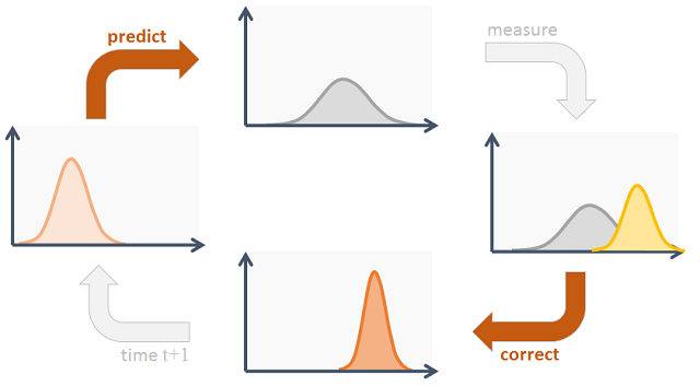
As we can see in the image above, the Kalman filter works recursively. First, we take current readings to predict the current state, then we use the measurements and update our predictions. So, it essentially boils down to inferring a new distribution (the predictions) from the previous state distribution and the measurement distribution.

The complete mathematical formulation and derivations concerning the Kalman filter are not covered in this post. However, it is recommended for you to go through them. You can read more on this link if you have enough mathematical background.

Kalman filter works best for linear systems with Gaussian processes involved. In our case, the tracks hardly leave the linear realm, and also, most methods and even noise fall into the Gaussian realm. So, the problem is suited for the use of Kalman filters.

Deep Learning based Object Tracking Approaches

Deep Regression Networks:

One of the early methods that used deep learning for single object tracking was Deep Regression Networks (ECCV, 2016). A model was trained on a dataset consisting of videos with labeled target frames. The objective of the model is to track a given object from the given image crop.

To achieve this, they use a two-frame CNN architecture which uses both the current and the previous frame to regress on to the object accurately:

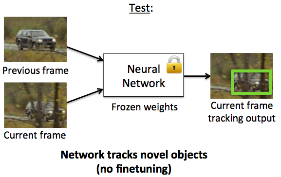
As shown in the above figure, we take the crop from the previous frame based on the predictions and define a "Search region" in the current structure based on that crop. Now the network is trained to regress for the object in this search region. The network architecture is simple with CNN's followed by Fully connected layers that directly give us the bounding box coordinates.

ROLO - Recurrent Yolo:

ROLO Recurrent Yolo (ISCAS 2016) - an elegant way to track objects using deep CNN. A slightly modified YOLO detector with an attached recurrent LSTM unit at the end helps track objects by capturing the Spatio-temporal features. Here is the architecture:

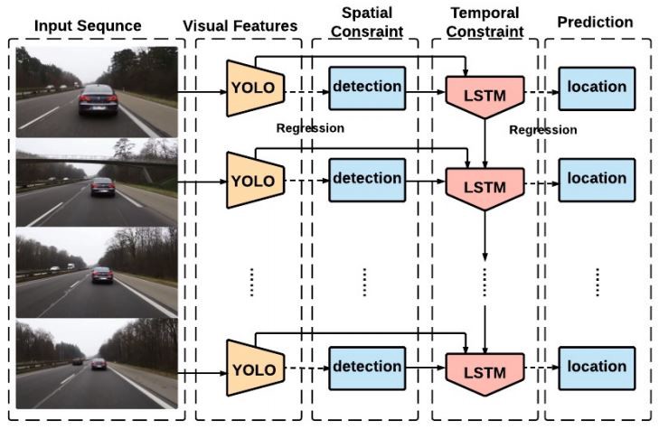
As shown in the above image, the architecture is quite simple. The Detections from YOLO (bounding boxes) are concatenated with the feature vector from a CNN-based feature extractor (We can either re-use the YOLO backend or use a specialized feature extractor). Now, this concatenated feature vector, which represents most of the spatial information related to the current object, along with the information on the previous state, is passed onto the LSTM cell.

The output of the cell now accounts for both spatial and temporal information. This simple trick of using CNN's for feature extraction and LSTM's, for bounding box predictions, greatly improved tracking challenges. The disadvantage of this method is that it's pretty hard to train the LSTM network.

Deep SORT

The most popular and widely used object tracking framework is Deep SORT (Simple Real-time Tracker).

In the Deep Sort tracker, the Kalman filter is a crucial component. Kalman tracking scenario is defined on the eight-dimensional state space (u, v, a, h, u', v', a', h') that contains the bounding box center position (u, v), are centers of the bounding boxes, a is the aspect ratio and h, the height of the image. The other variables are the respective velocities of the variables.

Note that variables have only absolute position and velocity factors since we assume a simple linear velocity model. The Kalman filter helps us factor in the noise in the detection and uses prior state in predicting a good fit for bounding boxes.

For each detection, we create a "Track", that has all the necessary state information. It also has a parameter to track and delete tracks that had their last successful detection long back, as those objects would have left the scene. To eliminate duplicate tracks, there is a minimum number of detections threshold for the first few frames.

When we have the new bounding boxes tracked from the Kalman filter, the next problem is associating new detections with the latest predictions. Since they are processed independently, the assignment problem comes because we have no idea how to associate track_i with incoming detection_k.

To solve this, we need a distance metric to quantify the association and an efficient algorithm to associate the data.

Deep Sort authors decided to use the squared Mahalanobis distance (effective metric when dealing with distributions) to incorporate the uncertainties from the Kalman filter. This metric is more accurate than euclidean distance as we effectively measure the distance between 2 distributions (everything is under the Kalman filter). Thresholding this distance can give us a perfect idea of the actual associations. In this case, the authors offered to use the standard Hungarian algorithm, a very effective and straightforward combinatorial optimization algorithm that solves the assignment problem.

The appearance feature vector:

Up to this point, we have an object detector giving us detections, Kalman filter tracking detections, and giving us missing tracks, and the Hungarian algorithm solving the association problem.

Despite the effectiveness of the Kalman filter, it fails in many real-world scenarios like occlusions, different viewpoints, etc.

So, to improve this, the authors of Deep SORT introduced another distance metric based on the "appearance" of the object.

So, the authors first built a classifier over the dataset, trained it till it achieved a reasonably good accuracy, and then stripped the final classification layer. Assuming a classical architecture, we will be left with a dense layer producing a single feature vector, waiting to be classified. That feature vector becomes our "appearance descriptor" of the object.

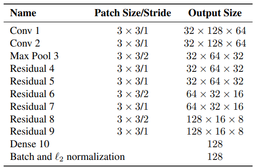
The "Dense 10" layer shown in the above pic will be our appearance feature vector for the given crop. Once trained, we need to pass all the crops of the detected bounding box from the image to this network and obtain the "128x1" dimensional feature vector. The updated distance metric will be:

$D=Lambda*D_k+(1-Lambda)*D_a$

Where D_k is the Mahalanobis distance, D_a is the cosine distance between the appearance feature vectors, and Lambda is the weighting factor.

Simple distance metrics combined with powerful deep learning techniques are all that is needed to make Deep Sort elegant and one of the most common object tracking tools.

Code Implementation:

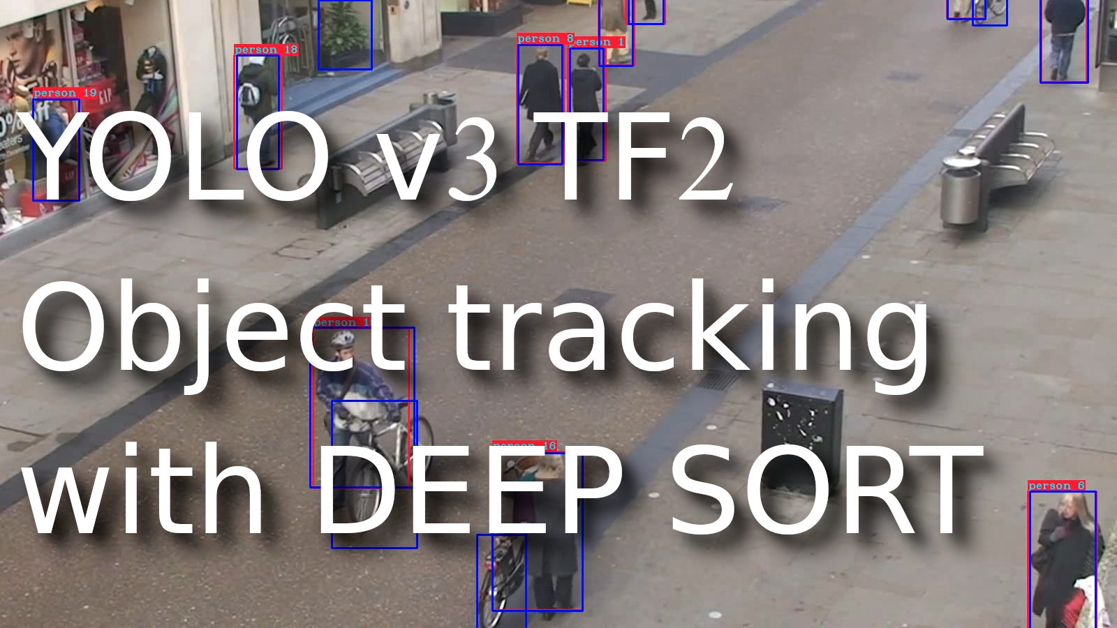
In this tutorial, I will implement our generic object tracker on the pre-trained (trained on COCO dataset) YOLOv3 model.

First, you should clone my GitHub repository and follow the setup instructions from the same repository REAMDE.md file. If you have issues, follow my past YOLOv3 tutorial (links can be found at the end of this tutorial).

Since we are interested in creating an object tracker and not a detector, we shall use video or real-time camera detection outputs to receive a series of frames.

The deep_sort folder in the repo has the original deep sort implementation, complete with the Kalman filter, Hungarian algorithm, and feature extractor. Originally it was written to work with TensorFlow 1.x. I had to modify the original files slightly to make them work with TensorFlow 2.

Let's look at my object_tracker.py script:

import os
import cv2
import numpy as np
import tensorflow as tf
from yolov3.yolov3 import Create_Yolov3
from yolov3.utils import load_yolo_weights, image_preprocess, postprocess_boxes, nms, draw_bbox, read_class_names
import time
from yolov3.configs import *

from deep_sort import nn_matching
from deep_sort.detection import Detection
from deep_sort.tracker import Tracker
from deep_sort import generate_detections as gdet

input_size = YOLO_INPUT_SIZE
Darknet_weights = YOLO_DARKNET_WEIGHTS
if TRAIN_YOLO_TINY:
    Darknet_weights = YOLO_DARKNET_TINY_WEIGHTS

video_path   = "./IMAGES/test.mp4"

yolo = Create_Yolov3(input_size=input_size)
load_yolo_weights(yolo, Darknet_weights) # use Darknet weights

def Object_tracking(YoloV3, video_path, output_path, input_size=416, show=False, CLASSES=YOLO_COCO_CLASSES, score_threshold=0.3, iou_threshold=0.45, rectangle_colors='', Track_only = []):
    # Definition of the parameters
    max_cosine_distance = 0.5
    nn_budget = None
    
    #initialize deep sort object
    model_filename = 'model_data/mars-small128.pb'
    encoder = gdet.create_box_encoder(model_filename, batch_size=1)
    metric = nn_matching.NearestNeighborDistanceMetric("cosine", max_cosine_distance, nn_budget)
    tracker = Tracker(metric)

    times = []

    if video_path:
        vid = cv2.VideoCapture(video_path) # detect on video
    else:
        vid = cv2.VideoCapture(0) # detect from webcam

    # by default VideoCapture returns float instead of int
    width = int(vid.get(cv2.CAP_PROP_FRAME_WIDTH))
    height = int(vid.get(cv2.CAP_PROP_FRAME_HEIGHT))
    fps = int(vid.get(cv2.CAP_PROP_FPS))
    codec = cv2.VideoWriter_fourcc(*'XVID')
    out = cv2.VideoWriter(output_path, codec, fps, (width, height)) # output_path must be .mp4

    NUM_CLASS = read_class_names(CLASSES)
    key_list = list(NUM_CLASS.keys()) 
    val_list = list(NUM_CLASS.values())
    while True:
        _, img = vid.read()

        try:
            original_image = cv2.cvtColor(img, cv2.COLOR_BGR2RGB)
            original_image = cv2.cvtColor(original_image, cv2.COLOR_BGR2RGB)
        except:
            break
        image_data = image_preprocess(np.copy(original_image), [input_size, input_size])
        image_data = tf.expand_dims(image_data, 0)
        
        t1 = time.time()
        pred_bbox = YoloV3.predict(image_data)
        t2 = time.time()

        times.append(t2-t1)
        times = times[-20:]
        
        pred_bbox = [tf.reshape(x, (-1, tf.shape(x)[-1])) for x in pred_bbox]
        pred_bbox = tf.concat(pred_bbox, axis=0)

        bboxes = postprocess_boxes(pred_bbox, original_image, input_size, score_threshold)
        bboxes = nms(bboxes, iou_threshold, method='nms')

        # extract bboxes to boxes (x, y, width, height), scores and names
        boxes, scores, names = [], [], []
        for bbox in bboxes:
            if len(Track_only) !=0 and NUM_CLASS[int(bbox[5])] in Track_only or len(Track_only) == 0:
                boxes.append([bbox[0].astype(int), bbox[1].astype(int), bbox[2].astype(int)-bbox[0].astype(int), bbox[3].astype(int)-bbox[1].astype(int)])
                scores.append(bbox[4])
                names.append(NUM_CLASS[int(bbox[5])])

        # Obtain all the detections for the given frame.
        boxes = np.array(boxes) 
        names = np.array(names)
        scores = np.array(scores)
        features = np.array(encoder(original_image, boxes))
        detections = [Detection(bbox, score, class_name, feature) for bbox, score, class_name, feature in zip(boxes, scores, names, features)]

        # Pass detections to the deepsort object and obtain the track information.
        tracker.predict()
        tracker.update(detections)

        # Obtain info from the tracks
        tracked_bboxes = []
        for track in tracker.tracks:
            if not track.is_confirmed() or track.time_since_update > 1:
                continue 
            bbox = track.to_tlbr() # Get the corrected/predicted bounding box
            class_name = track.get_class() #Get the class name of particular object
            tracking_id = track.track_id # Get the ID for the particular track
            index = key_list[val_list.index(class_name)] # Get predicted object index by object name
            tracked_bboxes.append(bbox.tolist() + [tracking_id, index]) # Structure data, that we could use it with our draw_bbox function

        ms = sum(times)/len(times)*1000
        fps = 1000 / ms

        # draw detection on frame
        image = draw_bbox(original_image, tracked_bboxes, CLASSES=CLASSES, tracking=True)
        image = cv2.putText(image, "Time: {:.1f} FPS".format(fps), (0, 30), cv2.FONT_HERSHEY_COMPLEX_SMALL, 1, (0, 0, 255), 2)

        # draw original yolo detection
        #image = draw_bbox(image, bboxes, CLASSES=CLASSES, show_label=False, rectangle_colors=rectangle_colors, tracking=True)

        #print("Time: {:.2f}ms, {:.1f} FPS".format(ms, fps))

        if output_path != '': out.write(image)
        if show:
            cv2.imshow('output', image)
            if cv2.waitKey(25) & 0xFF == ord("q"):
                cv2.destroyAllWindows()
                break

    cv2.destroyAllWindows()

Object_tracking(yolo, video_path, '', input_size=input_size, show=True, iou_threshold=0.1, rectangle_colors=(255,0,0), Track_only = [])

Same as in object detector; first, we initialize our YOLOv3 model, then we import necessary functions for our Deep Sort tracker.

Unlike my other functions in this project, which I put in the yolov3/utils.py script, I now create Object_tracking in the same file. We call this function in the following way:

Object_tracking(yolo, video_path, '', input_size=input_size, show=True, iou_threshold=0.1, rectangle_colors=(255,0,0), Track_only = [])

Where:

• YOLO is our YOLOv3 model;
• video_path is our video path, and if there is no path, it will use a web camera;
• input_size, show, iou_threshold=0.1, rectangle_colors are apparent parameters, which don't need an explanation. Otherwise, check my past tutorials;
• Track_only is used to define specific objects to track, for example, Track_only = ["person"]. Then our tracker will track only persons.

Talking about the Tracking, model_filename = 'model_data/mars-small128.pb' loads a CNN pre-trained deep_SORT tracking model. The function "tracker=Tracker(metric)" is one of the most important elements. A tracker is an object of the class Tracker defined in the deep_sort library that takes care of creation, keeping track, and eventual deletion of all tracks.

I am not going to explain code step by step, only at the abstract level. Deep Sort Detection requires boxes input in the following format (x, y, width, height), but our YOLOv3 outputs detections as (x_min, y_min, x_max, y_max), so we do a conversion.

The whole tracking is done in two lines:

tracker.predict() 

tracker.update(detections)

In other lines, we do operations with data. We can look into object tracking example (Tracking only the people), where I test the deep_sort framework on the test.mp4 video:

This is only a short gif from my results. If you want to see more, check my YouTube tutorial above.

Training custom feature extractor:

Since the original deep sort focused on the MARS dataset based on people, the feature extractor is trained on the human dataset. This means that this object tracking model works best to track people. It doesn't mean that our object tracker won't work on a custom object detector; simply, it won't work as well as it could. To get the best out of this tracking method, you should train an equivalent feature extractor for your custom objects.

But in this tutorial, I am not covering the training part. To train the deep association metric paper authors on their GitHub, refer to https://github.com/nwojke/cosine_metric_learning approach, provided as a separate repository.

Conclusion:

I hope this tutorial post has helped you gain a comprehensive understanding of the core ideas and components in object tracking. Also, I gave you a fully working code to test object tracking that you might use for your project. I have just one request, if you try this code on your project, mention me in your project. Also, it would be interesting to see what problem to solve you use it, so don't hesitate to comment on this post, on YouTube, or even write me an email! Now it's enough reading; go to my GitHub, clone repository, and try everything yourself!