YOLOv3 is one of the most popular real-time object detectors in Computer Vision. If you heard something more popular, I would like to hear it.
I showed you how to use YOLO v3 object detection with the TensorFlow 2 application and train Mnist custom object detection in my previous tutorials. At the end of the tutorial, I promised to show you how to train custom object detection. It was a challenging task, but I found a way to do that. However, before training a custom object detector, we must know where we may get a custom dataset or how we should label it. So, in this tutorial, I will show you where you could get a labeled dataset, how to prepare it for training, and finally, how to train it!
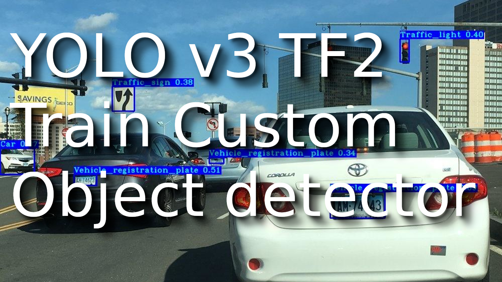
In this step-by-step tutorial, I will start with a simple case of training a 7-class object detector (we could use this method to get a dataset for every detector you may use). Therefore, I will build a Vehicle registration plate, Traffic sign, Traffic light, Car, Bus, Truck, and Person object detector.
1. Dataset:
As with any deep learning task, the first most crucial task is to prepare the training dataset. Dataset is the fuel that runs any deep learning model.
I will use images from Google's OpenImagesV6 dataset, publicly available online like in my past tutorials. It is a massive dataset with more than 600 different categories of an object. The dataset contains the bounding box, segmentation, or relationship annotations for these objects. As a whole, the dataset is more than 600GB in size, but we will download the images and classes only needed for our custom detector.
So, we have a link to this large dataset, but it's not explained how we should download the images and labels we need. Should we download them one by one? No, there is a fantastic OIDv4 ToolKit from GitHub with a full explanation of how to use it.
This Toolkit makes our life easier when we train a custom object detection model with popular objects and don't know where to get labeled images. This Toolkit allows downloading images from OID v6 seamlessly. The installation is easy and clearly explained in the readme file. The Toolkit is loaded with a variety of options. For example, the OIDv4 Toolkit allows us to download almost any particular class of interest from the given database. You can explore this dataset and check if there is a class you need for custom detection.
The Toolkit can be downloaded from the link I mentioned above or cloned by the following command:
git clone https://github.com/pythonlessons/OIDv4_ToolKit.git
If you installed requirements from my original project, you could skip the following step. Otherwise, the first thing you should do is install the necessary packages:
pip install -r OIDv4_ToolKit/requirements.txt
2. Using Toolkit:
At first start, you will be asked to download class-descriptions-boxable.csv (contains the name of all 600+ classes with their corresponding 'LabelName'), test-annotations-bbox.csv and train-annotations-bbox.csv (the file contains one bounding box (bbox for short) coordinates for one image. It also has this bbox's Label Name and current image's ID from the validation set of OIDv6) files to OID/csv_folder directory.
3. Downloading database images:
First, we should check if the database has an appropriate image class we need? Usually, I go to the OIDv6 page -> click on explore and find my needed class in a search tab. In my example, I will search for "Vehicle registration plate", "Traffic sign", "Traffic light", "Car", "Bus", "Truck", and "Person". To download all of them, we can use OIDv4_ToolKit. First, open the OIDv4_ToolKit directory: cd OIDv4_ToolKit, and from there, open the terminal. In a terminal, write the following command:
python main.py downloader --classes 'Vehicle registration plate' 'Traffic sign' 'Traffic light' Car Bus Truck Person --type_csv train --limit 2000
I will download 2000 training images for each class and place them in the train folder with this command. As I mentioned before, if you are using this for the first time, this will first download the train-annotations-bbox.csv CSV file and download the requested images from the specified class.
After it finished downloading the training dataset, do the same for the test dataset:
python main.py downloader --classes 'Vehicle registration plate' 'Traffic sign' 'Traffic light' Car Bus Truck Person --type_csv test --limit 200
After downloading the test and train dataset, the folders structure should look following:
TensorFlow-2.x-YOLOv3
│    ...
│    train.py
│    detection_custom.py
│    ...
└─── OIDv4_ToolKit
    │
    └─── OID
        │
        └─── csv_folder
        │   │
        │   └─── class-descriptions-boxable.csv
        │   │
        │   └─── test-annotations-bbox.csv
        │   │
        │   └─── train-annotations-bbox.csv
        │
        └─── OID
            │
            └─── Dataset
                │
                └─── train
                │   │
                │   └─── Bus, Car, Person, ...
                │
                └─── test
                    │
                    └─── Bus, Car, Person, ...
4. Converting label files to XML:
If you open one of the label files, you might see classes and coordinates of points in type of this: "name_of_the_class left top right bottom", where each coordinate is denormalized. So, the four different values correspond to the actual number of pixels of the related image.
So, we need to convert the text annotations format to XML. You may ask why we should convert it to XML? The XML format is quite popular and often used in other object detection algorithms, so I wrote a script to do this conversion. If you follow this tutorial and have the same file structure as I mentioned above, in the tools folder is the oid_to_pascal_voc_xml.py script. Run this script, and after it finishes conversion, you should find .xml files created.
5. Converting XML to YOLO v3 file structure:
First, to train a Yolo v3 model there are requirements how annotation file should look:
- One row for one image;
- Row format: image_file_path box1 box2 … boxN;
- Box format: x_min,y_min,x_max,y_max,class_id x_min2,y_min2,…;
- Here is an example:
path/to/img1.jpg 50,100,150,200,0 30,50,200,120,3
path/to/img2.jpg 120,300,250,600,2
…
We should have our .xml files prepared from the above 4th step or manually labeled images. To train our custom object detection model, we need an annotations file and class file. These files will be created with XML_to_YOLOv3.py script in the tools folder, same as in the 4th step; run this script. After conversion finishes, you should find Dataset_names.txt, Dataset_train.txt, and Dataset_test.txt files in the model_data folder.
6. Change Yolo v3 configurations:
Now you need to change the configs.py file to the following:
# YOLO options
YOLO_DARKNET_WEIGHTS        = "./model_data/yolov3.weights"
YOLO_COCO_CLASSES           = "./model_data/coco.names"
YOLO_STRIDES                = [8, 16, 32]
YOLO_IOU_LOSS_THRESH        = 0.5
YOLO_ANCHOR_PER_SCALE       = 3
YOLO_MAX_BBOX_PER_SCALE     = 100
YOLO_INPUT_SIZE             = 416
YOLO_ANCHORS                = [[[10,  13], [16,   30], [33,   23]],
                               [[30,  61], [62,   45], [59,  119]],
                               [[116, 90], [156, 198], [373, 326]]

# Train options
TRAIN_CLASSES               = "./model_data/Dataset_names.txt"
TRAIN_ANNOT_PATH            = "./model_data/Dataset_train.txt"
TRAIN_LOGDIR                = "./log"
TRAIN_BATCH_SIZE            = 8
TRAIN_INPUT_SIZE            = 416
TRAIN_DATA_AUG              = True
TRAIN_TRANSFER              = True
TRAIN_FROM_CHECKPOINT       = False
TRAIN_LR_INIT               = 1e-4
TRAIN_LR_END                = 1e-6
TRAIN_WARMUP_EPOCHS         = 2
#TRAIN_EPOCHS                = 30
TRAIN_EPOCHS                = 100

# TEST options
TEST_ANNOT_PATH             = "./model_data/Dataset_test.txt"
TEST_BATCH_SIZE             = 4
TEST_INPUT_SIZE             = 416
TEST_DATA_AUG               = False
TEST_DECTECTED_IMAGE_PATH   = ""
TEST_SCORE_THRESHOLD        = 0.3
TEST_IOU_THRESHOLD          = 0.45
Now start the training process with the following terminal command from the main TensorFlow-2.x-YOLOv3 folder:
python train.py
After a while, I recommend you checking Tensorboard to track the training process:
tensorboard --logdir=log
7. Transfer learning or train from zero?
Transfer learning is a technique to reuse the already pre-trained model on a new problem. It's viral in deep learning because it can train deep neural networks with comparatively little data and a much shorter time. This is very useful since most real-world problems typically do not have millions of labeled data points to train such complex models.
In transfer learning, the knowledge of an already trained machine learning model is applied to a different but related problem. For example, if you trained a simple classifier to predict whether an image contains a car, you could use the knowledge that the model gained during its training to recognize other objects like a truck.
With transfer learning, we try to exploit what has been learned in one task to improve generalization in another. We transfer the weights that a network has learned at "task A" to a new "task B."
The general idea is to use the knowledge a model has learned from a task with a lot of available labeled training data in a new task that doesn't have much data. Instead of starting the learning process from scratch, we begin with patterns learned from solving a related task.
Transfer learning is mainly used in computer vision and natural language processing tasks like sentiment analysis due to the massive computational power required.
Transfer learning has become quite popular with neural networks that require vast amounts of data and computational power.
In configs.py, you may see the line: TRAIN_TRANSFER; this is used to use transfer learning or not. This is how transfer learning looks in code:
if TRAIN_TRANSFER:
    Darknet = Create_Yolov3(input_size=input_size)
    load_yolo_weights(Darknet, Darknet_weights) # use darknet weights
yolo = Create_Yolov3(input_size=input_size, training=True, CLASSES=TRAIN_CLASSES)
if TRAIN_FROM_CHECKPOINT:
    try:
        yolo.load_weights(TRAIN_FROM_CHECKPOINT)
    except ValueError:
        print("Shapes are incompatible, transfering Darknet weights")
        TRAIN_FROM_CHECKPOINT = False
if TRAIN_TRANSFER and not TRAIN_FROM_CHECKPOINT:
    for i, l in enumerate(Darknet.layers):
        layer_weights = l.get_weights()
        if layer_weights != []:
            try:
                yolo.layers[i].set_weights(layer_weights)
            except:
                print("skipping", yolo.layers[i].name)
First, we create a model with original weights, then we create our custom model and copy all the weights from original model layers to custom model layers which are the same.
To better understand why we use transfer learning, I trained (on GTX1080TI) two models with the same ('Vehicle registration plate' 'Traffic sign' 'Traffic light' Car Bus Truck Person) dataset.
First, here are the results from Tensorboard without transfer learning:
![]()
To evaluate our model performance, we look at total validation loss. This is why we need testing data while training. As you can see from this chart, we achieved the best results(lowest low) within 43 steps with an evaluation value of 7.724. To get this model, it took almost 27 hours of training.
Here are results from Tensorboard with transfer learning:
![]()
While using transfer learning, we achieved the best results within the 7th step of validation with an evaluation value of 6.614, which took only 3 hours. As you can see, after this point, the validation curve began to rise, which means that we started overfitting, and it's not getting better while training it. The only way to improve it is by getting more training data and using more augmentation techniques and other techniques.
To test your custom trained model, use detection_custom.py script, change image_path for your image in code.
Conclusion:
From this tutorial, we learned where and how to download custom training data, prepare data for training, and choose which model is best. In the next part, I will show you how to label your data and train custom object detection on your own labeled data.