When I started learning YOLO v3, I noticed that it's challenging to understand both the concept and implementation. Even though there are tons of blog posts and GitHub repositories about it, most are presented in complex architectures.

I am not going to cover how Yolo works in theory step by step. I'll try to cover more in detail all parts from the past tutorial and parts I missed last time. If you are interested, check my past tutorial, where I tried to explain a whole theory. However, I implemented it in TensorFlow 1.15. But more and more people write to me about errors because they try my code within TF 2.0 or above, so I decided that it's time to write YOLO v3 implementation to TensorFlow 2.

In this tutorial series, I will give you solutions on how to train the Yolo model for your custom dataset locally or even on Google Colab (received a lot of requests). Based on that experience, I will try to write code in this tutorial to make it easy and reusable for many beginners who just got started learning object detection. Without over-complicating things, you will be able to implement Yolo v3 in TensorFlow 2 simply with this tutorial.

Prerequisites

• Familiar with Python 3;
• Understand object detection and Convolutional Neural Networks (CNN);
• Basic TensorFlow usage.

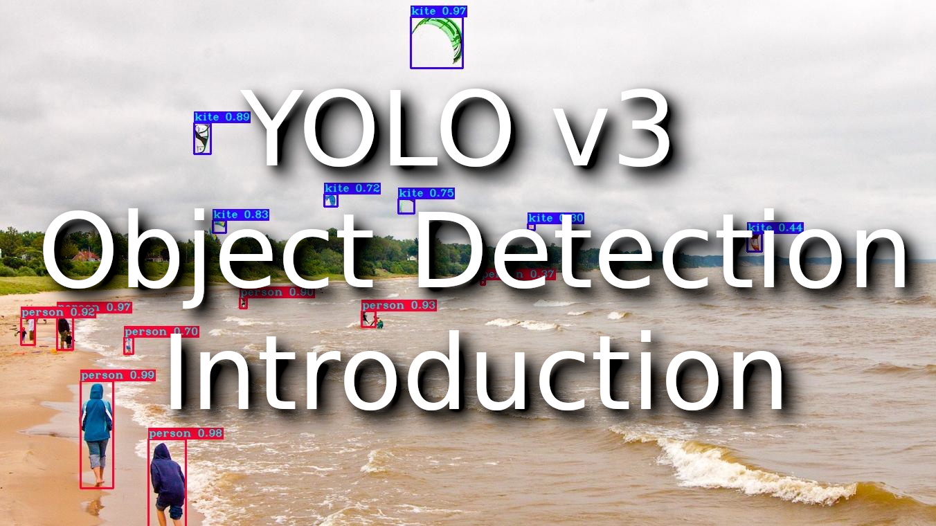
Introduction to YOLO algorithm

In 2015, Redmon J et al. Proposed the YOLO network, which is characterized by combining the candidate box generation and classification regression into a single step. Proposed architecture accelerated the speed of target detection, frame rate up to 45 fps! When predicting, the feature map is divided into 7x7 cells, and each cell is predicted, which significantly reduces the calculation complexity.

After a lapse of one year, Redmon J once again proposed YOLOv2. Compared with the previous generation, the mAP on the VOC2007 test set increased from 67.4% to 78.6%. However, because a cell is only responsible for predicting a single object facing the goal of overlap, the recognition was not good enough.

Finally, in April 2018, the author released the third version of YOLOv3.The mAP-50 on the COCO dataset increased from 44.0% of YOLOv2 to 57.9%. Compared with RetinaNet with 61.1% mAP, RetinaNet by default has an input size of 500x500. In this case, the detection speed is about 98 ms/frame, while YOLOv3 has 29 ms/frame when the input size is 416x416.

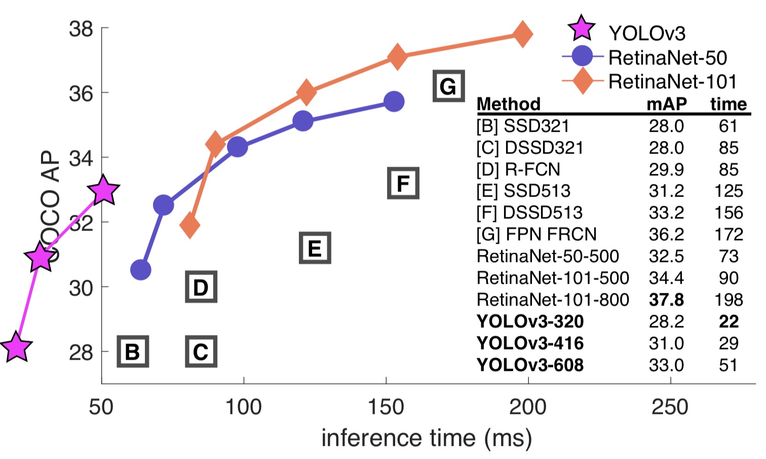The above picture is enough to prove that YOLOv3 has achieved a very high accuracy rate under the premise of ensuring speed.

YOLO v3 idea

The author treats the object detection problem as a regression problem in the YOLO algorithm and divides the image into an S × S grid. If the center of a target falls into a grid, the grid is responsible for detecting the target.

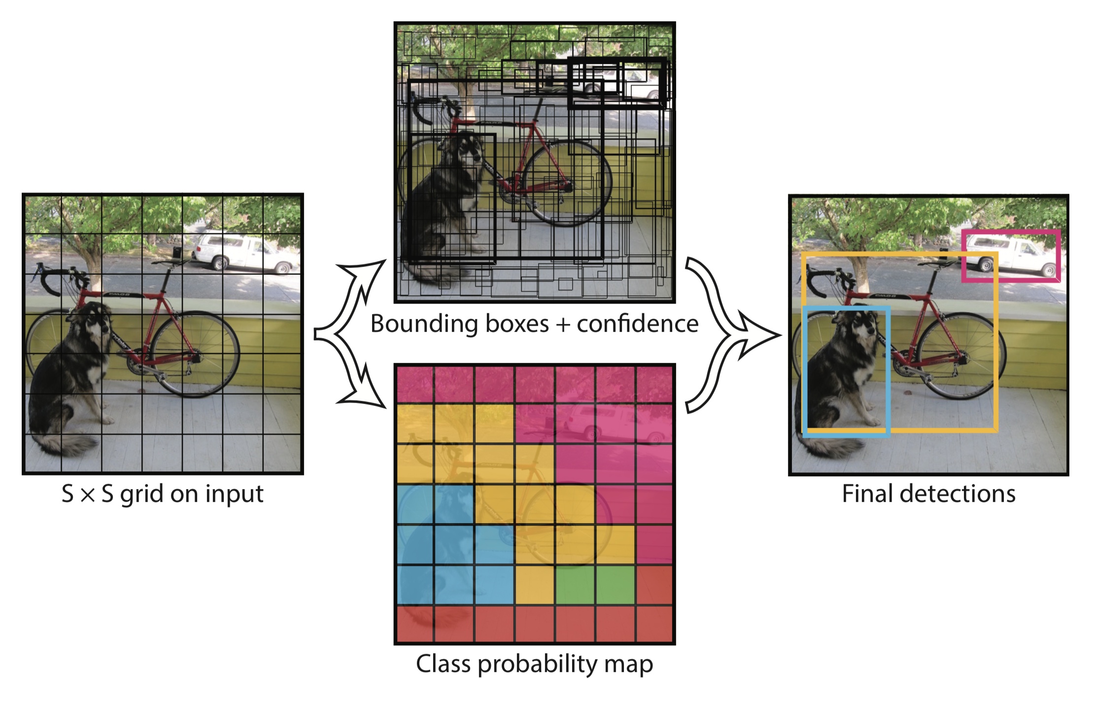Each grid will output a bounding box, confidence, and class probability map. Among them:

• The bounding box contains four values: x, y, w, h, (x, y) represents the center of the box. (W, h) defines the width and height of the box;
• Confidence indicates the probability of containing objects in this prediction box, which is the IoU value between the prediction box and the actual box;
• The class probability indicates the class probability of the object, and the YOLOv3 uses a two-class method.

YOLO v3 architecture

For those who don't have much experience with Yolo v3 or other object detections, I recommend reading my past tutorials and understanding how the algorithm works.

As its name suggests, YOLO (You Only Look Once) applies a single forward pass neural network to the whole image and predicts the bounding boxes and their class probabilities as well. This technique makes YOLO quite fast without losing a lot of accuracies.

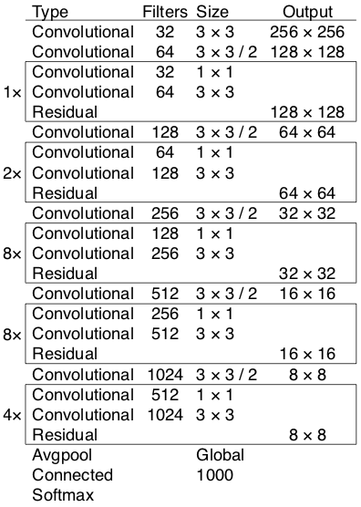
As mentioned in the original paper, YOLOv3 has 53 convolutional layers called Darknet-53 is shown in the bellow image. The figure is mainly composed of Convolutional and Residual structures. It should be noted that the last three layers Avgpool, Connected, and softmax layer, are used for classification training on the Imagenet dataset. When using the Darknet-53 layer to extract features from the picture, these three layers are not used.

Darknet-53 Implemented in code:

def darknet53(input_data):
    input_data = convolutional(input_data, (3, 3,  3,  32))
    input_data = convolutional(input_data, (3, 3, 32,  64), downsample=True)

    for i in range(1):
        input_data = residual_block(input_data,  64,  32, 64)

    input_data = convolutional(input_data, (3, 3,  64, 128), downsample=True)

    for i in range(2):
        input_data = residual_block(input_data, 128,  64, 128)

    input_data = convolutional(input_data, (3, 3, 128, 256), downsample=True)

    for i in range(8):
        input_data = residual_block(input_data, 256, 128, 256)

    route_1 = input_data
    input_data = convolutional(input_data, (3, 3, 256, 512), downsample=True)

    for i in range(8):
        input_data = residual_block(input_data, 512, 256, 512)

    route_2 = input_data
    input_data = convolutional(input_data, (3, 3, 512, 1024), downsample=True)

    for i in range(4):
        input_data = residual_block(input_data, 1024, 512, 1024)

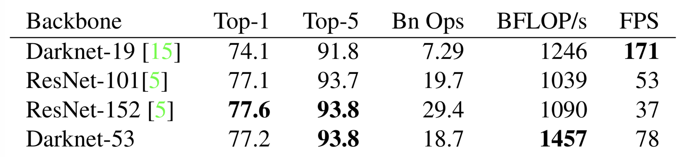
    return route_1, route_2, input_data

How strong is Darknet-53? Looking at the picture below, the author compares and concludes that Darknet-53 is comparable to the most advanced classifiers talking about accuracy, and it has fewer floating-point operations and the fastest calculation speed. Compared with ResNet-101, the speed of the Darknet-53 network is 1.5 times that of the former; although ReseNet-152 and its performance are similar, it takes more than two times.

In addition, Darknet-53 can also achieve the highest measurement floating-point operation per second, which means that the network structure can better use the GPU, thereby making it more efficient and faster.

But from the above Darknet-53 architecture figure, it's pretty impossible to understand or imagine how Yolo v3 works, so here is another figure with Yolo v3 architecture:

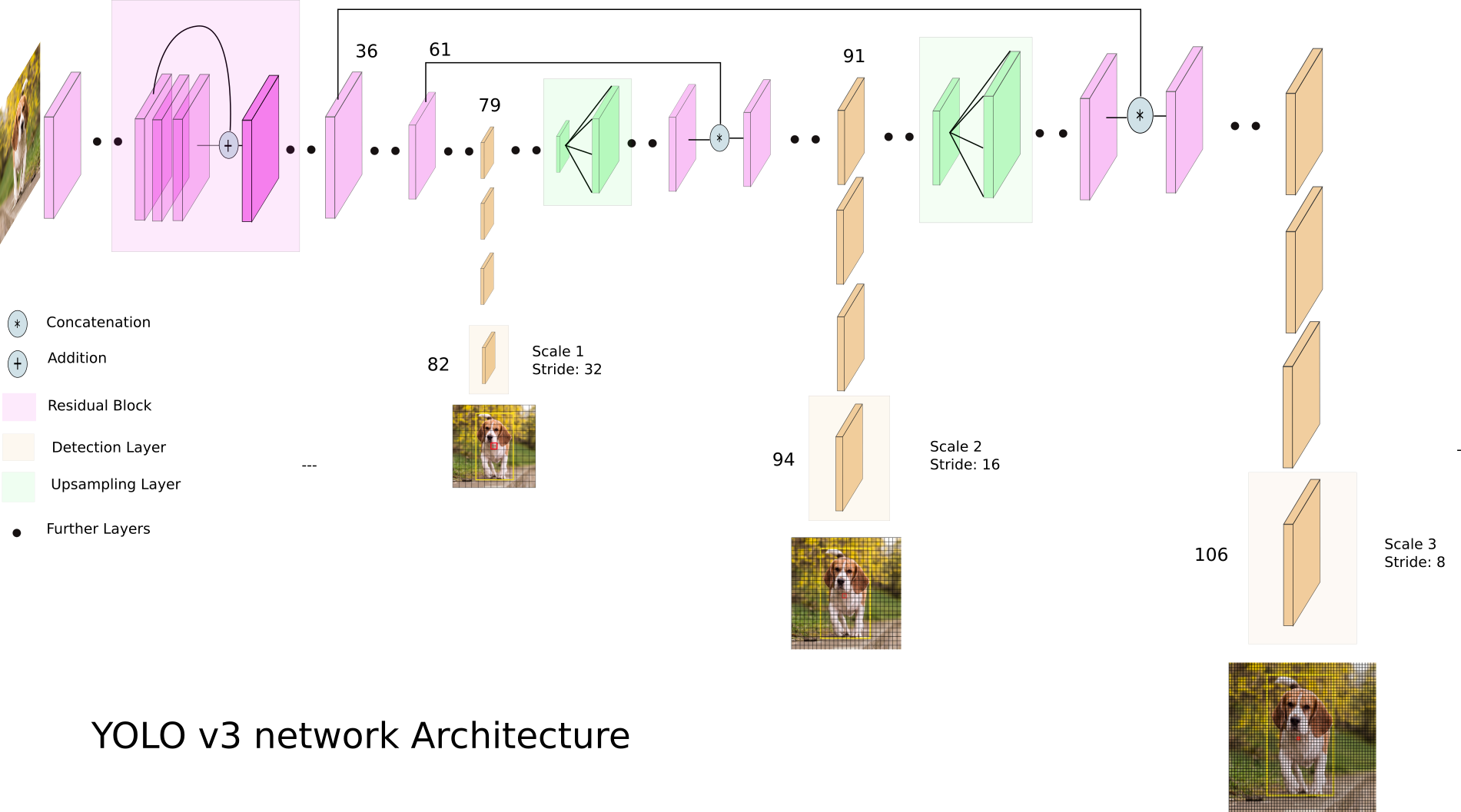
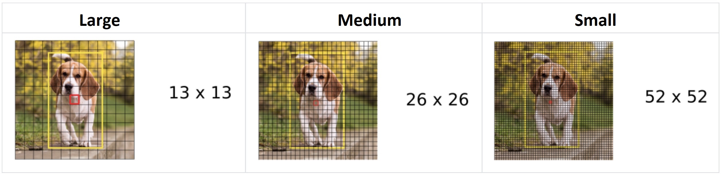
From the above architecture image, you can see that YOLO makes detection in 3 different scales to accommodate various objects sizes by using strides of 32, 16, and 8. This means, if we feed an input image of size 416x416, YOLOv3 will make detection on the scale of 13x13, 26x26, and 52x52.

YOLOv3 downsamples the input image into 13 x 13 and predicts the 82nd layer for the first scale. The 1st detection scale yields a 3-D tensor of size 13x13x255.

After that, YOLOv3 takes the feature map from layer 79 and applies one convolutional layer before upsampling it by a factor of 2 to have a size of 26 x 26. This upsampled feature map is then concatenated with the feature map from layer 61. The concatenated feature map is subjected to a few more convolutional layers until the 2nd detection scale is performed at layer 94. The second prediction scale produces a 3-D tensor of size 26 x 26 x 255.

The same design is again performed one more time to predict the 3rd scale. The feature map from layer 91 is added to one convolutional layer and is then concatenated with a feature map from layer 36. The final prediction layer is done at layer 106, yielding a 3-D tensor of size 52x52x255. In summary, Yolo predicts over three different scales detection, so if we feed an image of size 416x416, it produces three different output shape tensor, 13x13x255, 26x26x255, and 52x52x255.

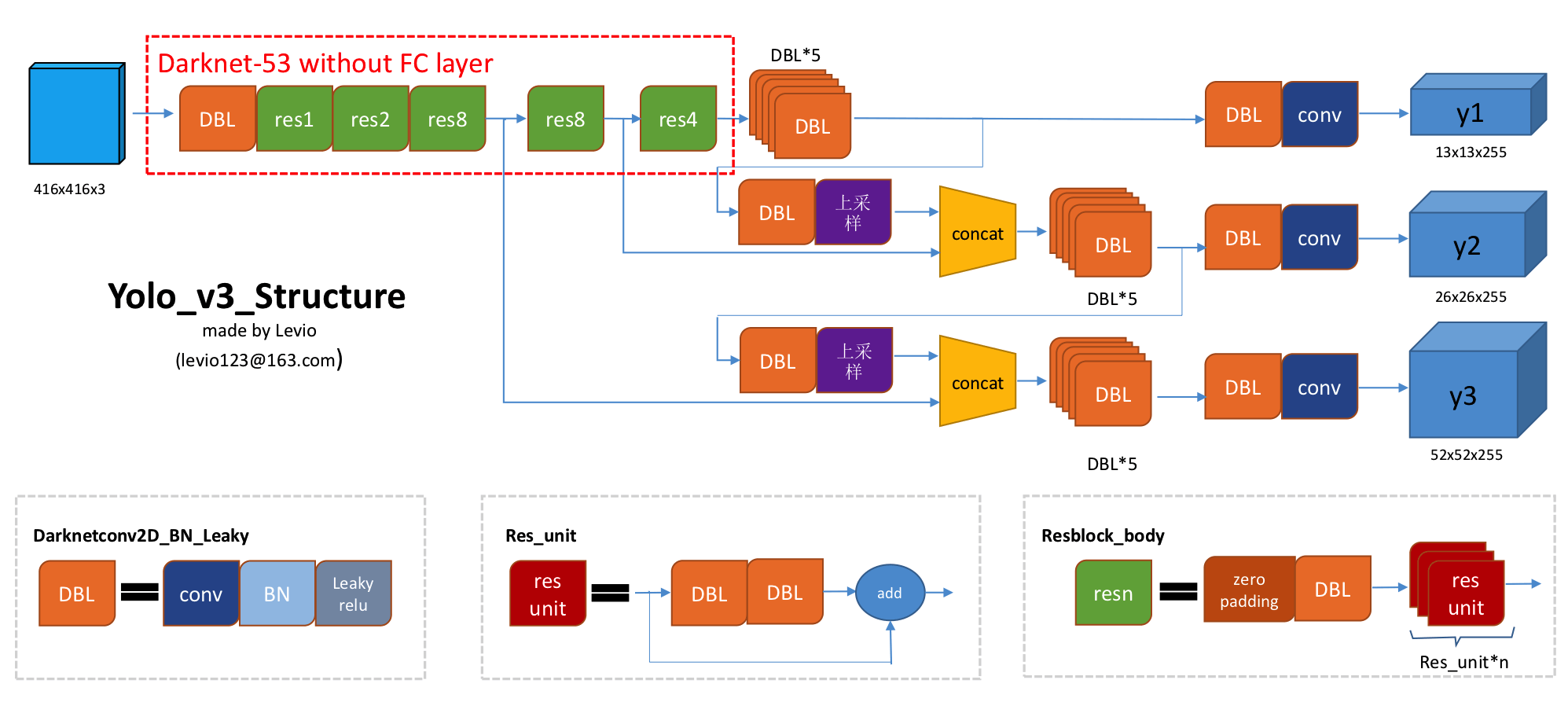
But still, seeing Darknet-53 and Yolo v3 structure, we can't fully understand all layers. This is why I have one more figure with the overall architecture of the YOLOv3 network. The picture below shows that the input picture of size 416x416 gets three branches after entering the Darknet-53 network. These branches undergo a series of convolutions, upsampling, merging, and other operations. Three feature maps with different sizes are finally obtained, with shapes of [13, 13, 255], [26, 26, 255] and [52, 52, 255]:

Implemented in code:

def YOLOv3(input_layer, NUM_CLASS):
    # After the input layer enters the Darknet-53 network, we get three branches
    route_1, route_2, conv = darknet53(input_layer)
    # See the orange module (DBL) in the figure above, a total of 5 Subconvolution operation
    conv = convolutional(conv, (1, 1, 1024,  512))
    conv = convolutional(conv, (3, 3,  512, 1024))
    conv = convolutional(conv, (1, 1, 1024,  512))
    conv = convolutional(conv, (3, 3,  512, 1024))
    conv = convolutional(conv, (1, 1, 1024,  512))
    conv_lobj_branch = convolutional(conv, (3, 3, 512, 1024))

    # conv_lbbox is used to predict large-sized objects , Shape = [None, 13, 13, 255] 
    conv_lbbox = convolutional(conv_lobj_branch, (1, 1, 1024, 3*(NUM_CLASS + 5)), activate=False, bn=False)

    conv = convolutional(conv, (1, 1,  512,  256))
    # upsample here uses the nearest neighbor interpolation method, which has the advantage that the
    # upsampling process does not need to learn, thereby reducing the network parameter  
    conv = upsample(conv)

    conv = tf.concat([conv, route_2], axis=-1)
    conv = convolutional(conv, (1, 1, 768, 256))
    conv = convolutional(conv, (3, 3, 256, 512))
    conv = convolutional(conv, (1, 1, 512, 256))
    conv = convolutional(conv, (3, 3, 256, 512))
    conv = convolutional(conv, (1, 1, 512, 256))
    conv_mobj_branch = convolutional(conv, (3, 3, 256, 512))

    # conv_mbbox is used to predict medium-sized objects, shape = [None, 26, 26, 255]
    conv_mbbox = convolutional(conv_mobj_branch, (1, 1, 512, 3*(NUM_CLASS + 5)), activate=False, bn=False)

    conv = convolutional(conv, (1, 1, 256, 128))
    conv = upsample(conv)

    conv = tf.concat([conv, route_1], axis=-1)
    conv = convolutional(conv, (1, 1, 384, 128))
    conv = convolutional(conv, (3, 3, 128, 256))
    conv = convolutional(conv, (1, 1, 256, 128))
    conv = convolutional(conv, (3, 3, 128, 256))
    conv = convolutional(conv, (1, 1, 256, 128))
    conv_sobj_branch = convolutional(conv, (3, 3, 128, 256))

    # conv_sbbox is used to predict small size objects, shape = [None, 52, 52, 255]
    conv_sbbox = convolutional(conv_sobj_branch, (1, 1, 256, 3*(NUM_CLASS +5)), activate=False, bn=False)

    return [conv_sbbox, conv_mbbox, conv_lbbox]

Residual module

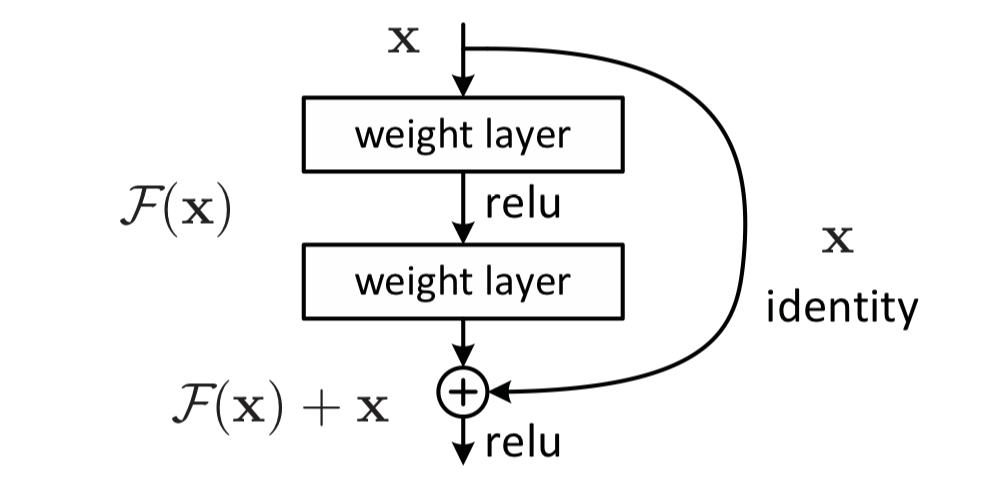
The most significant feature of the residual module is the use of a short cut mechanism (somewhat similar to the short circuit mechanism in the circuit) to alleviate the gradient disappearance problem caused by increasing the depth in the neural network, thereby making the neural network easier to optimize. It uses identity mapping to establish a direct correlation channel between input and output so that the network can concentrate on learning the residual between input and output.

Implementation in Python code:

def residual_block(input_layer, input_channel, filter_num1, filter_num2):
    short_cut = input_layer
    conv = convolutional(input_layer, filters_shape=(1, 1, input_channel, filter_num1))
    conv = convolutional(conv       , filters_shape=(3, 3, filter_num1,   filter_num2))

    residual_output = short_cut + conv
    return residual_output

Extract features

To know the prediction process of YOLO in detail, it is necessary first to understand feature maps and embeddings.

Feature map

When we talk about CNN networks, we always hear the word feature map. It is also called feature mapping. Simply put, the input image is convolved with the convolution kernel to obtain image features.

Generally speaking, when the CNN network extracts features from the bottom up of the image, the number of feature maps (in fact, the number of convolution kernels) will increase, and the spatial information will decrease. Its features will also become more and more abstract. For example, the famous VGG16 network, its feature map changes like this:

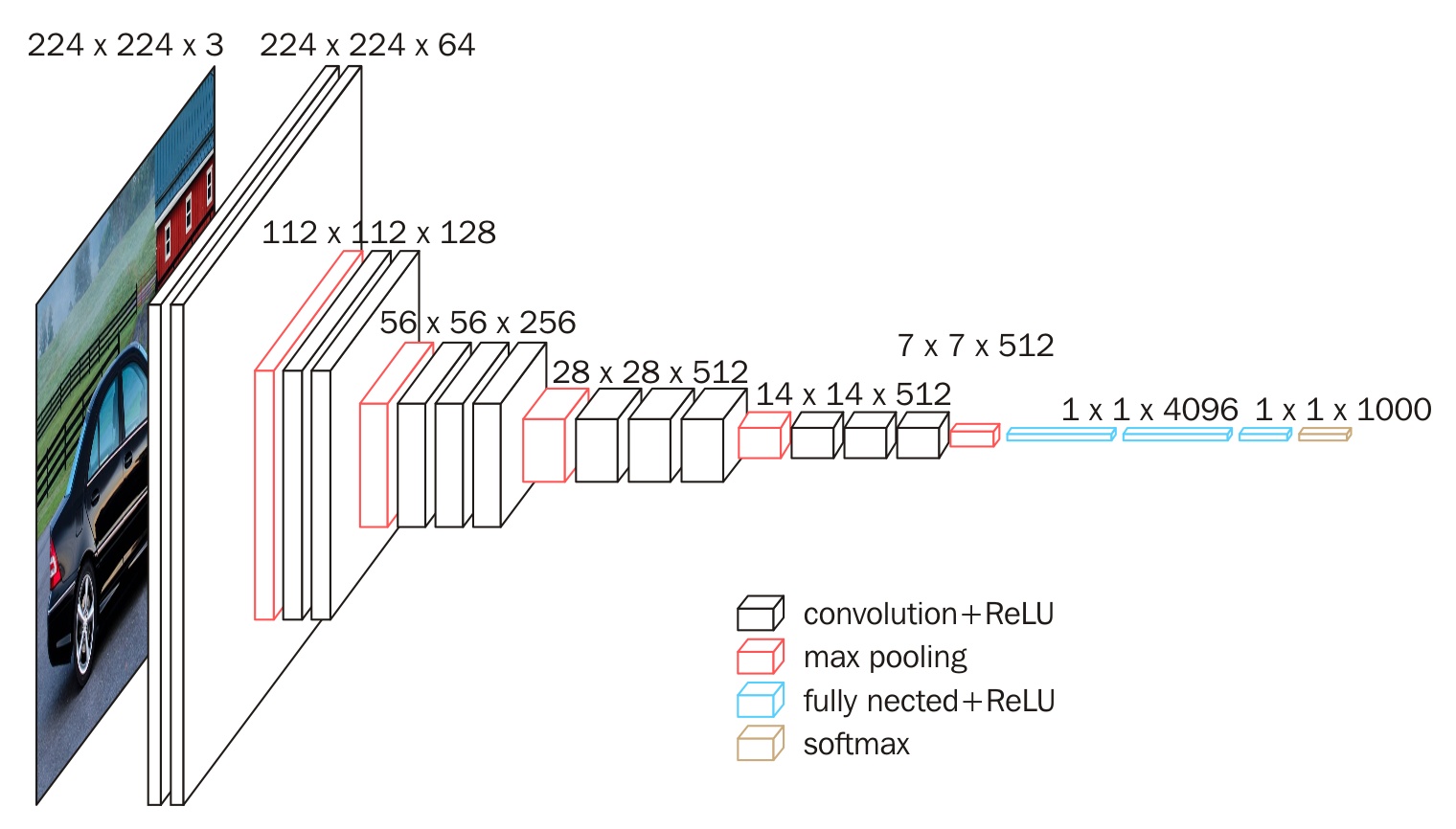The feature map is getting smaller and smaller in space but getting deeper and deeper in the channel size. This is the feature of VGG16.

Feature vector

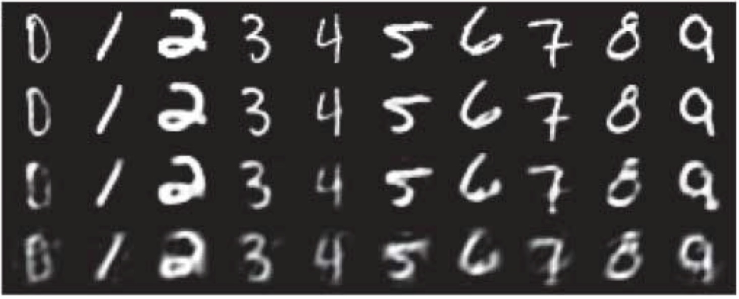
When it comes to feature maps, we can often hear them mentioned in the field of face recognition. As early as 2006, Hinton, the originator of deep learning, published a paper in "SCIENCE". Generally speaking, it is actually a feature map extracted by the last fully connected layer into a feature vector. For the first time, a self-encoding network was used to extract feature vectors (a 2D or 3D vector) from the Mnist handwritten digits. It is worth mentioning that this paper also opened the road to the rise of deep learning:

When CNN networks extract features from the bottom-up image, the resulting feature map is generally getting smaller and smaller in space size and getting deeper and deeper in channel size:

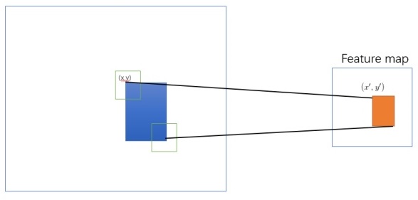This is related to the mapping of ROI (region of interest) to Feature Map. The information is the feature representation of the image information in the ROI area mapped on the CNN network. In the above picture: After an ROI in the original image is mapped in the CNN network space, the space size on the feature map will become smaller, or even a point, but the channel information of this point will be vibrant. Since the image pixels are closely connected in space, this results in significant redundancy in the area. Therefore, we often eliminate this redundancy by reducing the dimension in space and increasing the dimension in the channel, and try to obtain its most essential features in the smallest dimension:

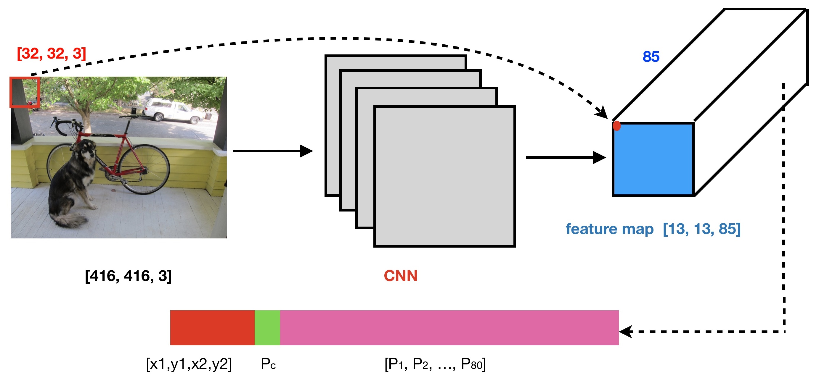For example, The red ROI in the upper left corner of the original image is mapped by CNN, and only one point is obtained on the feature map space, but this point has 85 channels. So, the dimension of ROI has changed from the original [32, 32, 3] to the current 85-dimension.

This is an 85-dimensional feature vector obtained after the CNN network performs feature extraction on the ROI. The first four dimensions of this feature vector represent candidate box information, the middle dimension represents the probability of judging the presence or absence of objects, and the following 80 dimensions represent the classification probability information for 80 categories.

Yolo v3 detection

Multi-scale detection

YOLO performs coarse, medium, and fine meshing of the input image to predict large, medium, and small objects, respectively. If the input picture size is 416X416, then the coarse, medium, and fine grid sizes are 13x13, 26x26, and 52x52, respectively. In this way, it is scaled by 32, 16, and 8 times in length and width, respectively:

Dimensions of the Bounding Box

The output of the three branches of the YOLOv3 network will be sent to the decode function to decode the channel information of the Feature Map. The dimensions of the bounding box are predicted by applying a log-space transformation to the output and then multiplying with an anchor: in the following picture: the black dotted box represents the a priori box (anchor), and the blue box represents the prediction box.

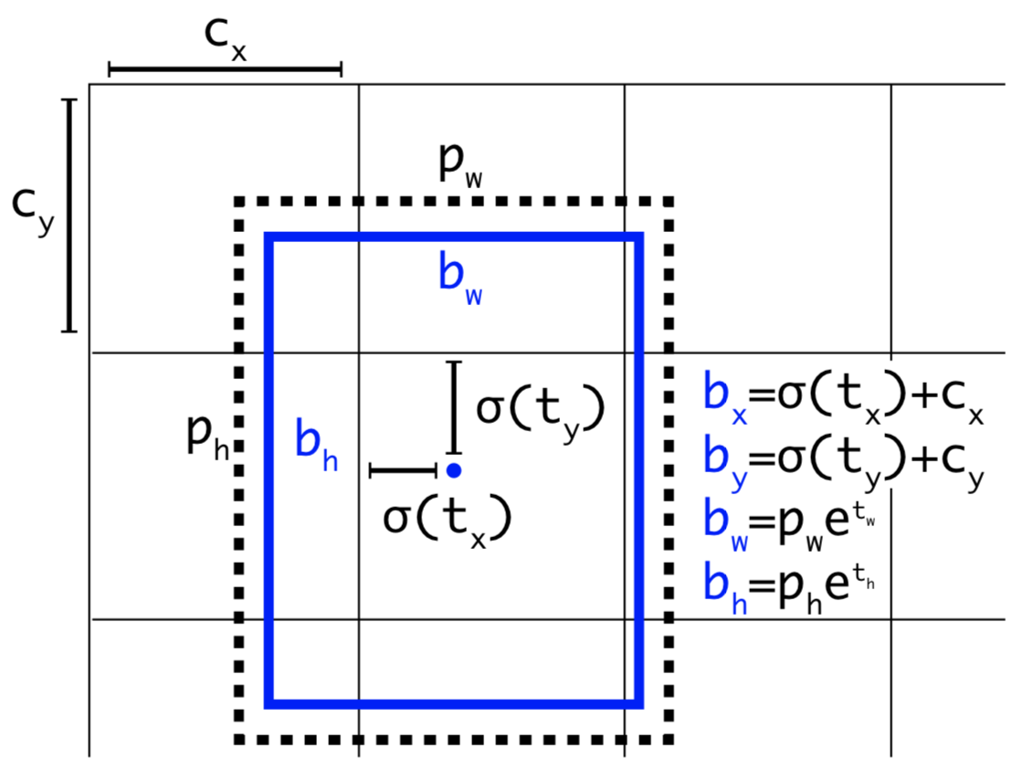
• b denotes the length and width of the prediction frame, respectively, and P represents the length and width of the a priori frame.
• t represents the offset of the object's center from the upper left corner of the grid, and C represents the coordinates of the upper left corner of the grid.

Implementation in Python code:

def decode(conv_output, NUM_CLASS, i=0):
    # where i = 0, 1 or 2 to correspond to the three grid scales  
    conv_shape       = tf.shape(conv_output)
    batch_size       = conv_shape[0]
    output_size      = conv_shape[1]

    conv_output = tf.reshape(conv_output, (batch_size, output_size, output_size, 3, 5 + NUM_CLASS))

    conv_raw_dxdy = conv_output[:, :, :, :, 0:2] # offset of center position     
    conv_raw_dwdh = conv_output[:, :, :, :, 2:4] # Prediction box length and width offset
    conv_raw_conf = conv_output[:, :, :, :, 4:5] # confidence of the prediction box
    conv_raw_prob = conv_output[:, :, :, :, 5: ] # category probability of the prediction box 

    # next need Draw the grid. Where output_size is equal to 13, 26 or 52  
    y = tf.range(output_size, dtype=tf.int32)
    y = tf.expand_dims(y, -1)
    y = tf.tile(y, [1, output_size])
    x = tf.range(output_size,dtype=tf.int32)
    x = tf.expand_dims(x, 0)
    x = tf.tile(x, [output_size, 1])

    xy_grid = tf.concat([x[:, :, tf.newaxis], y[:, :, tf.newaxis]], axis=-1)
    xy_grid = tf.tile(xy_grid[tf.newaxis, :, :, tf.newaxis, :], [batch_size, 1, 1, 3, 1])
    xy_grid = tf.cast(xy_grid, tf.float32)

    # Calculate the center position of the prediction box:
    pred_xy = (tf.sigmoid(conv_raw_dxdy) + xy_grid) * STRIDES[i]
    # Calculate the length and width of the prediction box:
    pred_wh = (tf.exp(conv_raw_dwdh) * ANCHORS[i]) * STRIDES[i]

    pred_xywh = tf.concat([pred_xy, pred_wh], axis=-1)
    pred_conf = tf.sigmoid(conv_raw_conf) # object box calculates the predicted confidence
    pred_prob = tf.sigmoid(conv_raw_prob) # calculating the predicted probability category box object

    # calculating the predicted probability category box object
    return tf.concat([pred_xywh, pred_conf, pred_prob], axis=-1)

NMS processing

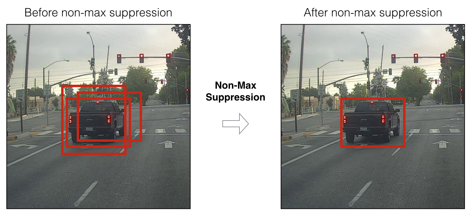
Non-Maximum Suppression, as the name implies, suppresses elements that are not maximal. NMS removes those bounding boxes that have a higher overlap rate and a lower score. The algorithm of NMS is straightforward, and the iterative process is as follows:

• Process 1: Determine whether the number of bounding boxes is greater than 0; if not, then end the iteration;
• Process 2: Select the bounding box A with the highest score according to the score order and remove it;
• Process 3: Calculate the IoU of this bounding box A and all remaining bounding boxes and remove those bounding boxes whose IoU value is higher than the threshold, repeat the above steps;

Implementation in Python code:

def nms(bboxes, iou_threshold, sigma=0.3, method='nms'):
    classes_in_img = list(set(bboxes[:, 5]))
    best_bboxes = []

    for cls in classes_in_img:
        cls_mask = (bboxes[:, 5] == cls)
        cls_bboxes = bboxes[cls_mask]
        # Process 1: Determine whether the number of bounding boxes is greater than 0 
        while len(cls_bboxes) > 0:
            # Process 2: Select the bounding box with the highest score according to score order A
            max_ind = np.argmax(cls_bboxes[:, 4])
            best_bbox = cls_bboxes[max_ind]
            best_bboxes.append(best_bbox)
            cls_bboxes = np.concatenate([cls_bboxes[: max_ind], cls_bboxes[max_ind + 1:]])
            # Process 3: Calculate this bounding box A and
            # Remain all iou of the bounding box and remove those bounding boxes whose iou value is higher than the threshold 
            iou = bboxes_iou(best_bbox[np.newaxis, :4], cls_bboxes[:, :4])
            weight = np.ones((len(iou),), dtype=np.float32)

            assert method in ['nms', 'soft-nms']

            if method == 'nms':
                iou_mask = iou > iou_threshold
                weight[iou_mask] = 0.0

            if method == 'soft-nms':
                weight = np.exp(-(1.0 * iou ** 2 / sigma))

            cls_bboxes[:, 4] = cls_bboxes[:, 4] * weight
            score_mask = cls_bboxes[:, 4] > 0.
            cls_bboxes = cls_bboxes[score_mask]

    return best_bboxes

In the end, all the bounding box A is what we want. Let's take a simple example: if the five bounding boxes and the scores are: A: 0.8, B: 0.05, C: 0.9, D: 0.5, E: 0.6, the set score threshold is 0.3, the calculation steps are as follows:

• Step 1: The number of bounding boxes is 5, satisfying the iteration conditions;
• Step 2: Select the bounding box A with the highest score and sort it out according to the score order;
• Step 3: Calculate the IoU of the bounding box A and the other four bounding boxes. Assume that the obtained IoU values are: B: 0.2, C: 0.7, D: 0.01, E: 0.08, and remove the bounding box C;
• Step 4: Now, only the bounding boxes B, D, E are left, satisfying the iteration conditions;
• Step 5: Select the bounding box D with the highest score according to the score order and remove it;
• Step 6: Calculate the IoU of the bounding box D and the other two bounding boxes. Assume that the obtained IoU values are: B: 0.06, E: 0.8, and remove the bounding box E;
• Step 7: Now only the bounding box B is left, satisfying the iteration conditions;
• Step 8: Select the bounding box B with the highest score according to the score order and remove it;
• Step 9: At this time, the number of bounding boxes is zero, and the iteration ends.

Finally, we get the bounding boxes A, B, and D, but the score of the bounding box B is very low, which indicates that the bounding box has no objects, so it should be discarded. In the YOLO algorithm, there are two cases of NMS processing: one is that all prediction frames are processed together with NMS, and the other is that NMS processing is performed separately for each category of prediction frames. In the latter case, there will be a phenomenon that the prediction box belongs to both category A and category B, which is more suitable for the case where multiple objects exist in a small cell simultaneously.

So, up to this point, we covered all the theories we needed for the simple use of YOLOv3. Now we can try to implement a simple detection example. In the next tutorial, I'll cover other functions required for custom object detector training.

Implementation

So this is only the first tutorial; not to make it too complicated, I'll do simple YOLOv3 object detection. To make it work with TensorFlow 2 we need to do the following steps:

• Construct and compile Yolov3 model in TensorFlow and Keras;
• Transfer weights from original Darknet weights to constructed model;
• Test object detection with image and video.

I will not show the complete code in this text tutorial. If you are interested in trying this, you can download it on GitHub.

First, you need to get my project:

git clone https://github.com/pythonlessons/TensorFlow-2.x-YOLOv3.git

Next, you may want to install the required python packages:

pip install -r ./requirements.txt

Now, download trained yolov3.weights from the project folder:

wget -P model_data https://pjreddie.com/media/files/yolov3.weights

Now you are ready to test Yolo v3 detection with the following script:

python detection_demo.py

If you did everything correctly, you should see the following image:

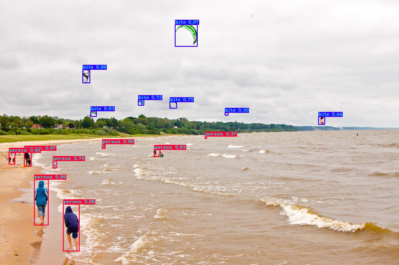Now you can play around and test your images by opening and editing the detection_demo.py script.

Conclusion:

That's it for this tutorial; in the next part, I will cover more theory related to custom Yolo v3 training, and of course, we'll train our first custom object detector. See you there!