In the previous tutorial, I showed you how to build a custom PyTorch model and train it in a wrapper to achieve modularity in our training pipeline. This tutorial will extend the previous tutorials to this one, using IAM Dataset. Before, I showed you how to use TensorFlow to train a model to recognize handwritten text from images. Now I'll do the same task, but with PyTorch!

The IAM Dataset comprises handwritten text images, and the target associated with each sample is the corresponding text string within the image. Since the IAM dataset is commonly employed as a benchmark for OCR systems, utilizing this example can provide a valuable foundation for constructing your own OCR system.

Handwriting recognition pertains to the process of converting handwritten text into text that machines can interpret. This technology is widely utilized in several applications, such as scanning documents, recognizing handwritten notes, and reading handwritten forms. Such applications include digitizing documents, analyzing handwriting, and automating the grading of exams. One approach to tackle handwriting recognition involves using a Connectionist Temporal Classification (CTC) loss function, which we have employed in my previous tutorials.

Prerequisites:

Before we begin, you will need to have the following software and packages installed:

• Python 3;
• torch (We will be using version 1.13.1 in this tutorial);
• mltu==1.0.2
• tensorboard==2.10.1
• onnx==1.12.0
• torchsummaryX

In this tutorial, we will look at code snippets used for training a handwritten word recognition model. The code is written in Python and uses PyTorch as its deep learning framework. The model is trained using the IAM dataset, a popular handwriting recognition dataset. The code uses several machine learning libraries and techniques to preprocess the data, augment it, and train a deep learning model.

We will start by looking at the code snippet line by line, understanding what each line does, and then we will discuss how to use this code for training a handwritten word recognition model.

Let's start with imports:

import os
import tarfile
from tqdm import tqdm
from io import BytesIO
from zipfile import ZipFile
from urllib.request import urlopen

import torch
import torch.optim as optim
from torchsummaryX import summary

from mltu.torch.model import Model
from mltu.torch.losses import CTCLoss
from mltu.torch.dataProvider import DataProvider
from mltu.torch.metrics import CERMetric, WERMetric
from mltu.torch.callbacks import EarlyStopping, ModelCheckpoint, TensorBoard, Model2onnx, ReduceLROnPlateau

from mltu.preprocessors import ImageReader
from mltu.transformers import ImageResizer, LabelIndexer, LabelPadding, ImageShowCV2
from mltu.augmentors import RandomBrightness, RandomRotate, RandomErodeDilate, RandomSharpen

from model import Network
from configs import ModelConfigs

The code imports several Python modules and libraries that are used in the training process:

• The os module is used for interacting with the operating system, e.g., reading or writing files, creating directories, etc.;
• The tarfile and zipfile modules are used for extracting files from archives, while urlopen is used to download files from the internet;
• The tqdm module is used for displaying progress bars during data processing, which is especially helpful when working with large datasets;
• The torch module is PyTorch's main module and is used for creating and training deep learning models.
• The DataProvider class is a custom class that is used to manage and preprocess the dataset. The ImageReader class reads images from the file system, and ImageResizer is used to resize the images.
• The LabelIndexer class converts text labels to integer indices, and LabelPadding pads the labels to a fixed length.
• The RandomBrightness, RandomRotate, RandomErodeDilate, and RandomSharpen classes are used for data augmentation. Data augmentation is a technique used to generate additional training data by applying transformations to the existing data. These techniques help to reduce overfitting and improve model performance;
• The Model class is a custom class that is used to train and evaluate the deep learning model;
• The CTCLoss class is a custom implementation of the Connectionist Temporal Classification loss function, which is commonly used for training text recognition models;
• The CERMetric and WERMetric classes are used to calculate character error rate (CER) and word error rate (WER) metrics during training;
• The EarlyStopping, ModelCheckpoint, TensorBoard, Model2onnx, and ReduceLROnPlateau classes are used as callbacks during training. Callbacks are functions that are called during training at specific intervals. They can be used to stop training early, save the model, visualize training metrics, and perform other useful functions;
• The Network is simply imported our PyTorch Neural Network model architecture, which you can find in the model.py file for more details. And the ModelConfigs are our training configurations as input image width and height, learning rate, vocabulary and, etc. Everything that is necessary for our training process.

Downloading and Extracting the Dataset

The next step is to download and extract the dataset:

def download_and_unzip(url, extract_to='Datasets', chunk_size=1024*1024):
    http_response = urlopen(url)

    data = b''
    iterations = http_response.length // chunk_size + 1
    for _ in tqdm(range(iterations)):
        data += http_response.read(chunk_size)

    zipfile = ZipFile(BytesIO(data))
    zipfile.extractall(path=extract_to)

dataset_path = os.path.join('Datasets', 'IAM_Words')
if not os.path.exists(dataset_path):
    download_and_unzip('https://git.io/J0fjL', extract_to='Datasets')

    file = tarfile.open(os.path.join(dataset_path, "words.tgz"))
    file.extractall(os.path.join(dataset_path, "words"))

The dataset is downloaded and extracted using the download_and_unzip function. The function takes the dataset URL as input and downloads it to the 'Datasets' directory. The function uses urlopen to open the URL and tqdm to show the progress bar while downloading the dataset. After the dataset is downloaded, it is extracted using ZipFile. The extracted dataset is saved in the 'Datasets/IAM_Words/words' directory.

Preprocessing the Dataset

After the dataset is downloaded and extracted, the next step is to preprocess the dataset:

dataset, vocab, max_len = [], set(), 0

# Preprocess the dataset by the specific IAM_Words dataset file structure
words = open(os.path.join(dataset_path, "words.txt"), "r").readlines()
for line in tqdm(words):
    if line.startswith("#"):
        continue

    line_split = line.split(" ")
    if line_split[1] == "err":
        continue

    folder1 = line_split[0][:3]
    folder2 = "-".join(line_split[0].split("-")[:2])
    file_name = line_split[0] + ".png"
    label = line_split[-1].rstrip('\n')

    rel_path = os.path.join(dataset_path, "words", folder1, folder2, file_name)
    if not os.path.exists(rel_path):
        print(f"File not found: {rel_path}")
        continue

    dataset.append([rel_path, label])
    vocab.update(list(label))
    max_len = max(max_len, len(label))

configs = ModelConfigs()

# Save vocab and maximum text length to configs
configs.vocab = "".join(sorted(vocab))
configs.max_text_length = max_len
configs.save()

This piece of code performs data preprocessing by parsing a words.txt file and populating three variables: dataset, vocab, and max_len. The dataset is a list that contains lists. Each inner list comprises a file path and its label. The vocab is a set of unique characters present in the labels. The max_len is the maximum length of the labels.

For each line in the file, the code executes the following tasks:

1. Skips the line if it starts with #;
2. Skips the line if the second element after splitting the line by space is "err";
3. Extracts the first three and eight characters of the filename and label, respectively;
4. Joins the dataset_path with the extracted folder names and filenames to form the file path;
5. Skips the line if the file path does not exist;
6. Otherwise, it adds the file path and label to the dataset list. Additionally, it updates the vocab set with the characters present in the label and updates the max_len variable to hold the maximum value of the current max_len and the length of the label;

After pre-processing the dataset, the code saves the vocabulary and the maximum text length to configs using the ModelConfigs class.

Prepare the data provider:

The IAM Words dataset contains images of handwritten text and their corresponding transcriptions. The preprocessing is done using the DataProvider class from the mltu.torch library:

# Create a data provider for the dataset
data_provider = DataProvider(
    dataset=dataset,
    skip_validation=True,
    batch_size=configs.batch_size,
    data_preprocessors=[ImageReader()],
    transformers=[
        # ImageShowCV2(), # uncomment to show images during training
        ImageResizer(configs.width, configs.height, keep_aspect_ratio=False),
        LabelIndexer(configs.vocab),
        LabelPadding(max_word_length=configs.max_text_length, padding_value=len(configs.vocab))
        ],
    use_cache=True,
)

The DataProvider class is initialized with the following parameters:

• dataset: The dataset to be used for training and validation;
• skip_validation: A boolean value indicating whether to skip validation or not;
• batch_size: The batch size for training the deep learning model;
• data_preprocessors: A list of data preprocessors to be applied to the dataset. In the given code, only ImageReader() is used, which reads the images from the file system;
• transformers: A list of transformers to be applied to the dataset. In the given code, the following transformers are used:
  • ImageResizer(): Resizes the images to the specified height and width;
  • LabelIndexer(): Converts the transcriptions to indices;
  • LabelPadding(): Pads the transcriptions with a padding value to make
• use_cache: flag whether to store our training data in RAM for faster preprocessing or not.

We can use way more functionality with this object, but that's the most important thing we need for our project right now.

We can use ImageShowCV2() function to visualize our images that are fed to data_provider while iterating our data_provider generator. Uncomment this line, and just after it, insert the following lines:

for _ in data_provider:
    pass

And now, if we run our script up to this point, we should see similar results on our screen:

Once the data provider has been created, the code splits it into training and validation sets using the split method:

# Split the dataset into training and validation sets
train_dataProvider, test_dataProvider = data_provider.split(split = 0.9)

Now that we have a split of our training and validation data, we need to add a few augmentation techniques to our training data provider that help us to train a better model:

# Augment training data with random brightness, rotation and erode/dilate
train_dataProvider.augmentors = [
    RandomBrightness(), 
    RandomErodeDilate(),
    RandomSharpen(),
    RandomRotate(angle=10), 
    ]

Create a PyTorch model:

Once the data providers have been created, we create a Network object, passing the length of the vocabulary and other configuration options, such as the activation function and dropout rate:

network = Network(len(configs.vocab), activation='leaky_relu', dropout=0.3)

It is not the topic to cover the model architecture, but if you are eager to check it out, go to the model.py file that is between tutorial files.

Then we create an optim.Adam object for the optimizer and an CTCLoss object for the loss function. The CTCLoss is used because the problem being solved is a character recognition problem where the length of the input and output sequence is not necessarily the same:

loss = CTCLoss(blank=len(configs.vocab))
optimizer = optim.Adam(network.parameters(), lr=configs.learning_rate)

If we are interested, we can print the summary of our model:

# uncomment to print network summary, torchsummaryX package is required
summary(network, torch.zeros((1, configs.height, configs.width, 3)))

This will produce as following results:

===================================================================================
                                Kernel Shape      Output Shape    Params  \
Layer
0_rb1.convb1.Conv2d_conv       [3, 16, 3, 3]  [1, 16, 32, 128]     448.0
1_rb1.convb1.BatchNorm2d_bn             [16]  [1, 16, 32, 128]      32.0
2_rb1.LeakyReLU_act1                       -  [1, 16, 32, 128]         -
3_rb1.convb2.Conv2d_conv      [16, 16, 3, 3]  [1, 16, 32, 128]     2.32k
4_rb1.convb2.BatchNorm2d_bn             [16]  [1, 16, 32, 128]      32.0
5_rb1.Conv2d_shortcut          [3, 16, 1, 1]  [1, 16, 32, 128]      64.0
6_rb1.LeakyReLU_act2                       -  [1, 16, 32, 128]         -
7_rb1.Dropout_dropout                      -  [1, 16, 32, 128]         -
8_rb2.convb1.Conv2d_conv      [16, 16, 3, 3]   [1, 16, 16, 64]     2.32k
9_rb2.convb1.BatchNorm2d_bn             [16]   [1, 16, 16, 64]      32.0
10_rb2.LeakyReLU_act1                      -   [1, 16, 16, 64]         -
11_rb2.convb2.Conv2d_conv     [16, 16, 3, 3]   [1, 16, 16, 64]     2.32k
12_rb2.convb2.BatchNorm2d_bn            [16]   [1, 16, 16, 64]      32.0
13_rb2.Conv2d_shortcut        [16, 16, 1, 1]   [1, 16, 16, 64]     272.0
14_rb2.LeakyReLU_act2                      -   [1, 16, 16, 64]         -
15_rb2.Dropout_dropout                     -   [1, 16, 16, 64]         -
16_rb3.convb1.Conv2d_conv     [16, 16, 3, 3]   [1, 16, 16, 64]     2.32k
17_rb3.convb1.BatchNorm2d_bn            [16]   [1, 16, 16, 64]      32.0
18_rb3.LeakyReLU_act1                      -   [1, 16, 16, 64]         -
19_rb3.convb2.Conv2d_conv     [16, 16, 3, 3]   [1, 16, 16, 64]     2.32k
20_rb3.convb2.BatchNorm2d_bn            [16]   [1, 16, 16, 64]      32.0
21_rb3.LeakyReLU_act2                      -   [1, 16, 16, 64]         -
22_rb3.Dropout_dropout                     -   [1, 16, 16, 64]         -
23_rb4.convb1.Conv2d_conv     [16, 32, 3, 3]    [1, 32, 8, 32]     4.64k
24_rb4.convb1.BatchNorm2d_bn            [32]    [1, 32, 8, 32]      64.0
25_rb4.LeakyReLU_act1                      -    [1, 32, 8, 32]         -
26_rb4.convb2.Conv2d_conv     [32, 32, 3, 3]    [1, 32, 8, 32]    9.248k
27_rb4.convb2.BatchNorm2d_bn            [32]    [1, 32, 8, 32]      64.0
28_rb4.Conv2d_shortcut        [16, 32, 1, 1]    [1, 32, 8, 32]     544.0
29_rb4.LeakyReLU_act2                      -    [1, 32, 8, 32]         -
30_rb4.Dropout_dropout                     -    [1, 32, 8, 32]         -
31_rb5.convb1.Conv2d_conv     [32, 32, 3, 3]    [1, 32, 8, 32]    9.248k
32_rb5.convb1.BatchNorm2d_bn            [32]    [1, 32, 8, 32]      64.0
33_rb5.LeakyReLU_act1                      -    [1, 32, 8, 32]         -
34_rb5.convb2.Conv2d_conv     [32, 32, 3, 3]    [1, 32, 8, 32]    9.248k
35_rb5.convb2.BatchNorm2d_bn            [32]    [1, 32, 8, 32]      64.0
36_rb5.LeakyReLU_act2                      -    [1, 32, 8, 32]         -
37_rb5.Dropout_dropout                     -    [1, 32, 8, 32]         -
38_rb6.convb1.Conv2d_conv     [32, 64, 3, 3]    [1, 64, 4, 16]   18.496k
39_rb6.convb1.BatchNorm2d_bn            [64]    [1, 64, 4, 16]     128.0
40_rb6.LeakyReLU_act1                      -    [1, 64, 4, 16]         -
41_rb6.convb2.Conv2d_conv     [64, 64, 3, 3]    [1, 64, 4, 16]   36.928k
42_rb6.convb2.BatchNorm2d_bn            [64]    [1, 64, 4, 16]     128.0
43_rb6.Conv2d_shortcut        [32, 64, 1, 1]    [1, 64, 4, 16]    2.112k
44_rb6.LeakyReLU_act2                      -    [1, 64, 4, 16]         -
45_rb6.Dropout_dropout                     -    [1, 64, 4, 16]         -
46_rb7.convb1.Conv2d_conv     [64, 64, 3, 3]    [1, 64, 4, 16]   36.928k
47_rb7.convb1.BatchNorm2d_bn            [64]    [1, 64, 4, 16]     128.0
48_rb7.LeakyReLU_act1                      -    [1, 64, 4, 16]         -
49_rb7.convb2.Conv2d_conv     [64, 64, 3, 3]    [1, 64, 4, 16]   36.928k
50_rb7.convb2.BatchNorm2d_bn            [64]    [1, 64, 4, 16]     128.0
51_rb7.LeakyReLU_act2                      -    [1, 64, 4, 16]         -
52_rb7.Dropout_dropout                     -    [1, 64, 4, 16]         -
53_rb8.convb1.Conv2d_conv     [64, 64, 3, 3]    [1, 64, 4, 16]   36.928k
54_rb8.convb1.BatchNorm2d_bn            [64]    [1, 64, 4, 16]     128.0
55_rb8.LeakyReLU_act1                      -    [1, 64, 4, 16]         -
56_rb8.convb2.Conv2d_conv     [64, 64, 3, 3]    [1, 64, 4, 16]   36.928k
57_rb8.convb2.BatchNorm2d_bn            [64]    [1, 64, 4, 16]     128.0
58_rb8.LeakyReLU_act2                      -    [1, 64, 4, 16]         -
59_rb8.Dropout_dropout                     -    [1, 64, 4, 16]         -
60_rb9.convb1.Conv2d_conv     [64, 64, 3, 3]    [1, 64, 4, 16]   36.928k
61_rb9.convb1.BatchNorm2d_bn            [64]    [1, 64, 4, 16]     128.0
62_rb9.LeakyReLU_act1                      -    [1, 64, 4, 16]         -
63_rb9.convb2.Conv2d_conv     [64, 64, 3, 3]    [1, 64, 4, 16]   36.928k
64_rb9.convb2.BatchNorm2d_bn            [64]    [1, 64, 4, 16]     128.0
65_rb9.LeakyReLU_act2                      -    [1, 64, 4, 16]         -
66_rb9.Dropout_dropout                     -    [1, 64, 4, 16]         -
67_lstm                                    -      [1, 64, 256]  198.656k
68_lstm_dropout                            -      [1, 64, 256]         -
69_output                          [256, 79]       [1, 64, 79]   20.303k
-----------------------------------------------------------------------------------
                         Totals
Total params           544.847k
Trainable params       544.847k
Non-trainable params        0.0
Mult-Adds             47.53456M
===================================================================================
Backend TkAgg is interactive backend. Turning interactive mode on.

And if we have a GPU on our device, its necessary to place our model on the GPU device:

# put on cuda device if available
if torch.cuda.is_available():
    network = network.cuda()

Now let's move on to the next section of the code, where the Model class is defined in the mltu.torch.model module. The Model class is a high-level interface that wraps the lower-level PyTorch functionality to make it easier to train and test neural network models. It takes care of all the boilerplate code required to train a neural network, such as forward and backward passes, loss computation, and parameter updates, allowing the user to focus on the model architecture and data.

# create callbacks
earlyStopping = EarlyStopping(monitor='val_CER', patience=20, mode="min", verbose=1)
modelCheckpoint = ModelCheckpoint(configs.model_path + '/model.pt', monitor='val_CER', mode="min", save_best_only=True, verbose=1)
tb_callback = TensorBoard(configs.model_path + '/logs')
reduce_lr = ReduceLROnPlateau(monitor='val_CER', factor=0.9, patience=10, verbose=1, mode='min', min_lr=1e-6)
model2onnx = Model2onnx(
    saved_model_path=configs.model_path + '/model.pt', 
    input_shape=(1, configs.height, configs.width, 3), 
    verbose=1,
    metadata={"vocab": configs.vocab}
    )

# create model object that will handle training and testing of the network
model = Model(network, optimizer, loss, metrics=[CERMetric(configs.vocab), WERMetric(configs.vocab)])
model.fit(
    train_dataProvider, 
    test_dataProvider, 
    epochs=1000, 
    callbacks=[earlyStopping, modelCheckpoint, tb_callback, reduce_lr, model2onnx]
    )

# Save training and validation datasets as csv files
train_dataProvider.to_csv(os.path.join(configs.model_path, 'train.csv'))
test_dataProvider.to_csv(os.path.join(configs.model_path, 'val.csv'))

The Model class takes four main arguments: network, optimizer, loss, and metrics. The Network is an instance of a PyTorch neural network model that takes input tensors and returns output tensors. Optimizer is an instance of a PyTorch optimizer that takes the network's parameters as input and updates them based on the gradients computed during backpropagation. Loss is an instance of a PyTorch loss function that computes the difference between the network's predictions and the actual labels. Metrics is a list of instances of custom metrics that evaluate the performance of the network on the validation set during training.

The Model class has several methods for training and testing the model. The fit method trains the model for a specified number of epochs using the training and validation data providers and applies the specified callbacks at each training stage. The evaluation method evaluates the performance of the model on a given dataset using the specified metrics. 

In the code, the Model object is instantiated with the Neural Network instance, the Adam optimizer, the CTCLoss loss function loss, and a list of two custom metrics: CERMetric and WERMetric. CERMetric computes the Character Error Rate (CER), which is the ratio of the number of incorrect characters to the total number of characters in the predictions. WERMetric computes the Word Error Rate (WER), which is the ratio of the number of incorrectly recognized words to the total number of words in the predictions.

Finally, the Model instance's fit method is called with the train_dataProvider and test_dataProvider datasets, the number of epochs set to 1000, and a list of five callbacks: earlyStopping, modelCheckpoint, tb_callback, reduce_lr, and model2onnx. These callbacks are defined in the mltu.torch.callbacks module and are used to save the best model based on validation loss, stop the training process early if the model's performance does not improve for a specified number of epochs, log the model's performance metrics using TensorBoard, reduce the learning rate when the model's performance plateaus, and save the model in the ONNX format for deployment.

At the end of the training process, the train_dataProvider dataset and the test_dataProvider dataset are saved as CSV files in the configs.model_path directory. These CSV files can be used for further analysis of the dataset and model performance.

Training performance on TensorBoard:

In the same way, as we do in TensorFlow, we can check the training and validation logs in Tensorboard. Its as simple as calling a tensorboard with the path to our logs folder, in my case:

Tensorboard --logdir Models\08_handwriting_recognition_torch\202303142139\logs

It gives us the link that we need to open:

Serving TensorBoard on localhost; to expose to the network, use a proxy or pass --bind_all
TensorBoard 2.10.1 at http://localhost:6006/ (Press CTRL+C to quit)

There we can analyze whole training and validation curves, and I am mostly interested in CER (Character Error Rate) curve:

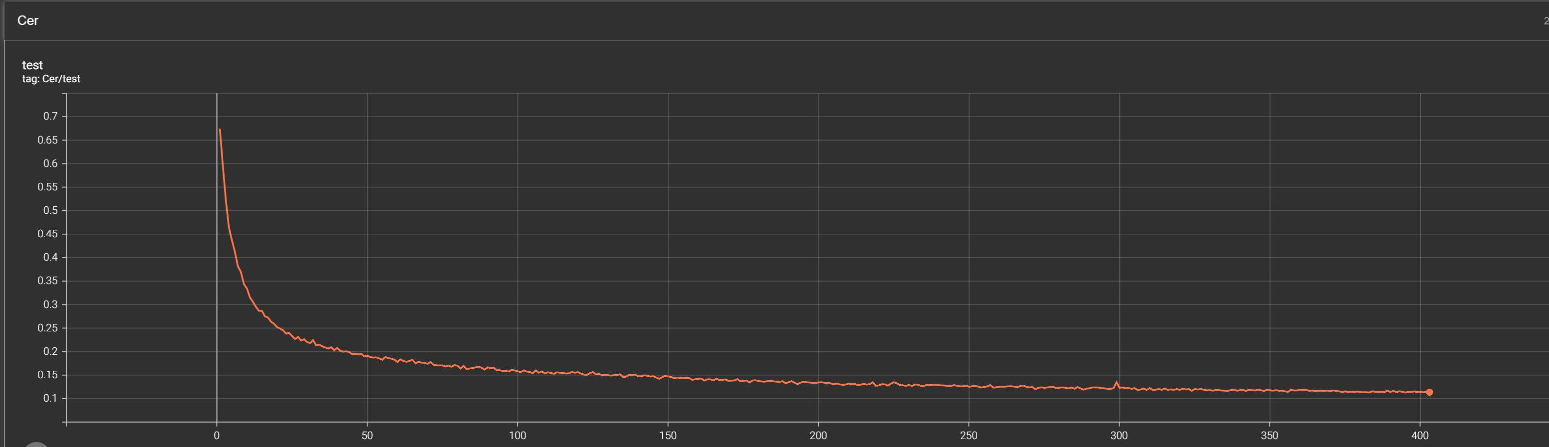
From the above (CER) curve, we can see that our model was definitely training as long as the curve kept decreasing. We can see that the whole training took around 400 training epochs, and the best model was saved somewhere around the 350th step. There it stays somewhere around 0.12 CER; that's not bad! This means that from a string, there is a chance that our model makes a mistake is around 12%. That comparably stunning results!

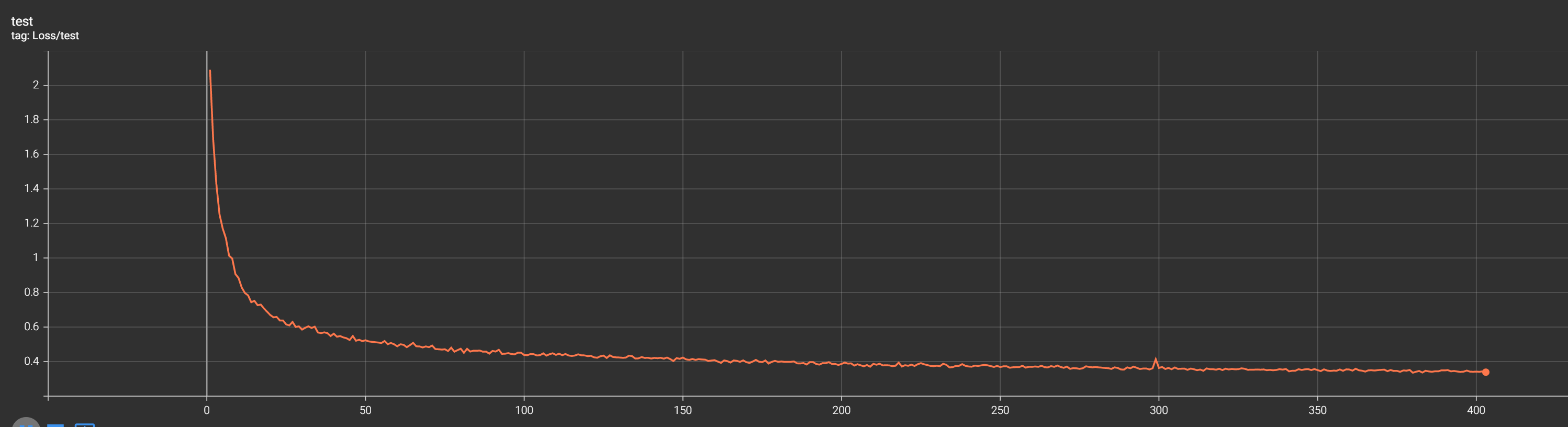
The above loss curve doesn't tell us any useful information apart from that it keeps decreasing, which means that our model keeps training.

Test-trained ONNX model:

My trained model was saved to  "Models/08_handwriting_recognition_torch/202303142139/model.onnx" onnx format, which allows us to load it with onnx inference and use it out of the box! As our training has finished, we want to test it to see actual predictions in string format. Here is the code to loop through our validation dataset:

import cv2
import typing
import numpy as np

from mltu.inferenceModel import OnnxInferenceModel
from mltu.utils.text_utils import ctc_decoder, get_cer

class ImageToWordModel(OnnxInferenceModel):
    def __init__(self, *args, **kwargs):
        super().__init__(*args, **kwargs)

    def predict(self, image: np.ndarray):
        image = cv2.resize(image, self.input_shape[:2][::-1])

        image_pred = np.expand_dims(image, axis=0).astype(np.float32)

        preds = self.model.run(None, {self.input_name: image_pred})[0]

        text = ctc_decoder(preds, self.vocab)[0]

        return text

if __name__ == "__main__":
    import pandas as pd
    from tqdm import tqdm

    model = ImageToWordModel(model_path="Models/08_handwriting_recognition_torch/202303142139/model.onnx")

    df = pd.read_csv("Models/08_handwriting_recognition_torch/202303142139/val.csv").values.tolist()

    accum_cer = []
    for image_path, label in tqdm(df):
        image = cv2.imread(image_path)

        prediction_text = model.predict(image)

        cer = get_cer(prediction_text, label)
        print(f"Image: {image_path}, Label: {label}, Prediction: {prediction_text}, CER: {cer}")

        accum_cer.append(cer)

    print(f"Average CER: {np.average(accum_cer)}")

The above code defines a class called ImageToWordModel that extends the OnnxInferenceModel class from the mltu.inferenceModel module. This class is designed to predict the word in an image of handwriting.

The predict method takes an input image and returns the predicted text by first resizing the image to the input shape of the model, running the image through the model, and then using a CTC decoder to decode the output predictions. The predicted text is returned by the predict method.

The __main__ block imports the pandas and tqdm modules and instantiates the ImageToWordModel class by passing the path to the ONNX model file. A CSV file containing image paths and their corresponding labels is read into a Pandas data frame, and the prediction method is called on each image in the data frame.

The predicted text is compared to the ground truth label for each image using the get_cer function from the mltu.utils.text_utils module to calculate the Character Error Rate (CER). The image path, ground truth label, predicted text, and CER is printed to the console. The CER values for all images are accumulated in a list, and the average CER is printed to the console after all images have been processed.

To use this code for your handwriting recognition task, you must provide your own ONNX model file and CSV file containing image paths and their corresponding labels. You could then modify the prediction method to perform any additional pre-processing or post-processing steps required by your specific task.

If I run the above script in the console, it gives me the following results:

...
Image: Datasets/IAM_Words/words/b05/b05-017/b05-017-03-03.png, Label: won't, Prediction: won't, CER: 0.0
Image: Datasets/IAM_Words/words/a01/a01-049u/a01-049u-07-06.png, Label: session, Prediction: sessicn, CER: 0.14285714285714285
Image: Datasets/IAM_Words/words/a02/a02-000/a02-000-07-00.png, Label: but, Prediction: but, CER: 0.0
Image: Datasets/IAM_Words/words/m02/m02-087/m02-087-06-02.png, Label: as, Prediction: as, CER: 0.0
Image: Datasets/IAM_Words/words/g06/g06-037j/g06-037j-07-01.png, Label: his, Prediction: his, CER: 0.0
Image: Datasets/IAM_Words/words/g06/g06-047i/g06-047i-02-09.png, Label: human, Prediction: human, CER: 0.0
Image: Datasets/IAM_Words/words/c03/c03-094c/c03-094c-08-03.png, Label: gaudy, Prediction: gaudy, CER: 0.0
Image: Datasets/IAM_Words/words/e04/e04-132/e04-132-01-04.png, Label: on, Prediction: on, CER: 0.0
Image: Datasets/IAM_Words/words/k02/k02-018/k02-018-04-01.png, Label: surprised, Prediction: supised, CER: 0.2222222222222222
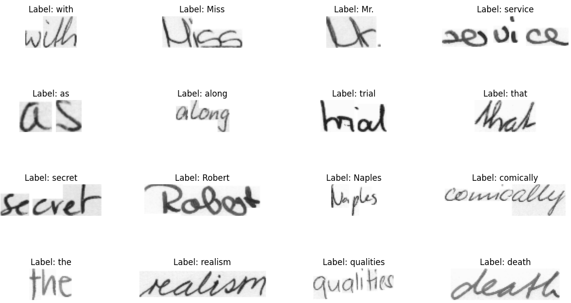
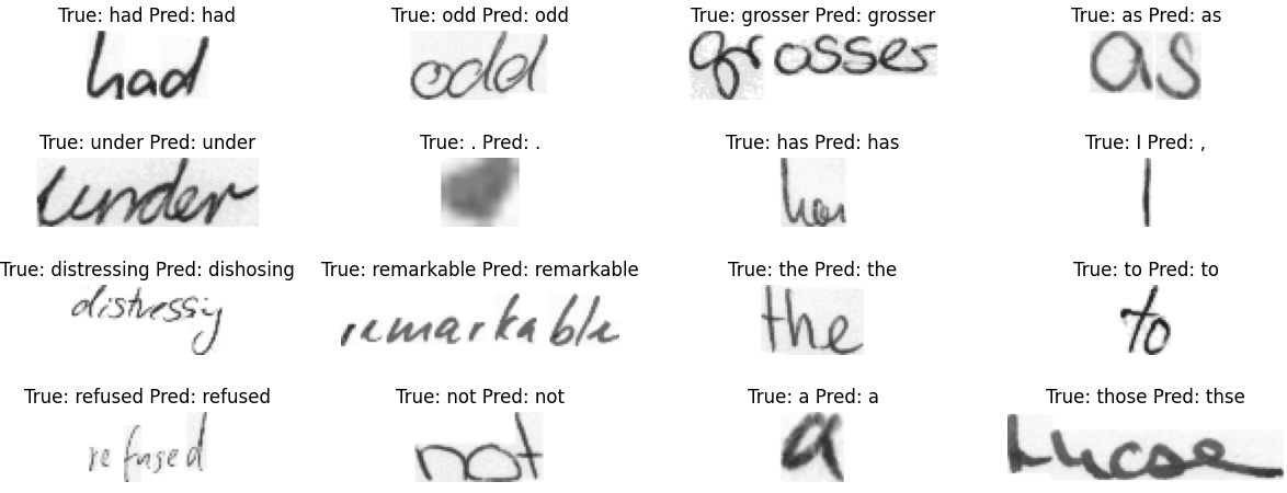
Average CER: 0.08829593383934714

Here we can see the actual label in the dataset and the predicted label. Also, it tells us the CER, and we can understand where it made any mistakes if it did. Here are a few images from my test dataset:

Conclusion:

In conclusion, this tutorial presented the implementation of a PyTorch model to recognize handwritten text from images using the IAM dataset. We used several machine learning techniques to preprocess the data, augment it, and train a deep learning model, including data augmentation and Connectionist Temporal Classification (CTC) loss function. The IAM dataset is a popular benchmark for OCR systems, making this tutorial an excellent starting point for building your OCR system. 

The tutorial also covered the importance of callbacks and the implementation of custom classes for managing and pre-processing the dataset, calculating evaluation metrics, and saving the model. Overall, this tutorial provided a comprehensive guide to building a handwritten word recognition model using PyTorch, which can be useful in several applications, including digitizing documents, analyzing handwriting, and automating the grading of exams.

The trained model used in this tutorial can be downloaded from this link.

The complete code for this tutorial you can find in this GitHub link.