Welcome to my other introduction tutorial on PyTorch! In this tutorial, I will show you how to use PyTorch to classify MNIST digits with convolutional neural networks. In previous tutorials, I demonstrated basic concepts using TensorFlow. However, this time, I will focus on PyTorch and explain how to transition from TensorFlow to PyTorch or where to begin. Before I get into the details, I will introduce PyTorch and its features.

PyTorch is an open-source machine-learning library based on the Torch library. It is primarily developed by Facebook's AI research division and is widely used for deep learning applications. In this tutorial, we will build a simple digit (MNIST) classifier using PyTorch. We will start by setting up our environment and loading the dataset. We will then define our model and train it on the dataset. Finally, we will test the model and make predictions.

First, let's talk about the differences between TensorFlow and PyTorch. PyTorch requires writing everything from scratch, which can take time. However, it offers more flexibility, making it a desirable option for some users. PyTorch has a lot of pre-built models, such as ResNet, which can be used for transfer learning. PyTorch also has better documentation and a more straightforward debugging process than TensorFlow.

This tutorial will consist of two parts:

Part 1: Setting up the Environment and Loading the Dataset

• Installing PyTorch and other dependencies
• Loading the MNIST dataset
• Preparing the dataset for training
• Visualizing the dataset

Part 2: Defining and Training the Model

• Defining the model architecture
• Setting up the training loop
• Training the model on the dataset
• Testing the model and making predictions

Prerequisites:

Before we begin, you will need to have the following software installed:

• Python 3;
• torch;
• torchsummary.

To start using PyTorch, you will need to install the CPU version "pip install torch". You don't need to worry about the GPU version, as this tutorial is relatively small, but if you want, you can find more information on the PyTorch website. 

Preparing the Dataset

After installation, we need to download the MNIST dataset. The code is specific and downloads the data from a given link. 

import os
import cv2
import numpy as np
from tqdm import tqdm
import requests, gzip, os, hashlib

import torch
import torch.nn as nn
import torch.optim as optim
from torchsummary import summary

from model import Net

# define path to store dataset
path='Datasets/mnist'
def fetch(url):
    if os.path.exists(path) is False:
        os.makedirs(path)

    fp = os.path.join(path, hashlib.md5(url.encode('utf-8')).hexdigest())
    if os.path.isfile(fp):
        with open(fp, "rb") as f:
            data = f.read()
    else:
        with open(fp, "wb") as f:
            data = requests.get(url).content
            f.write(data)
    return np.frombuffer(gzip.decompress(data), dtype=np.uint8).copy()

# load mnist dataset from yann.lecun.com, train data is of shape (60000, 28, 28) and targets are of shape (60000)
train_data = fetch("http://yann.lecun.com/exdb/mnist/train-images-idx3-ubyte.gz")[0x10:].reshape((-1, 28, 28))
train_targets = fetch("http://yann.lecun.com/exdb/mnist/train-labels-idx1-ubyte.gz")[8:]
test_data = fetch("http://yann.lecun.com/exdb/mnist/t10k-images-idx3-ubyte.gz")[0x10:].reshape((-1, 28, 28))
test_targets = fetch("http://yann.lecun.com/exdb/mnist/t10k-labels-idx1-ubyte.gz")[8:]

This code downloads specific files into "path='Datasets/mnist'". We will have training, validation, and validation target batches, with each training batch containing 60,000 images and validation containing 10,000 images.

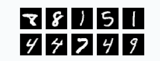
To visualize a few examples from our dataset, we can use the OpenCV python package:

# uncomment to show images from dataset using OpenCV
for train_image, train_target in zip(train_data, train_targets):
    train_image = cv2.resize(train_image, (400, 400))
    cv2.imshow("Image", train_image)
    # if Q button break this loop
    if cv2.waitKey(0) & 0xFF == ord('q'):
        break
cv2.destroyAllWindows()

We are resizing images to larger ones simply for visualization because originally, images are 28 by 28 size in pixels, which is very small. 

If we checked our data's shape, we would see the training shape (60000, 28, 28) and the validation shape (10000, 28, 28). 

We will normalize these images between zero and one. This will make it easier for the neural network to learn. Additionally, we will expand the dimensions of the images to prepare them for the convolutional layer. 

# define training hyperparameters
n_epochs = 5
batch_size_train = 64
batch_size_test = 64
learning_rate = 0.001

# reshape data to (items, channels, height, width) and normalize to [0, 1]
train_data = np.expand_dims(train_data, axis=1) / 255.0
test_data = np.expand_dims(test_data, axis=1) / 255.0

If we checked the shape of our data after these steps, we would see that the training shape now is (60000, 1, 28, 28) and the validation shape (10000, 1, 28, 28). 

Still, we can't train the model on 60000 images at once. We need to create smaller training batches because our CPU or GPU usually can't handle such a large batch. So, we split our data into sets of 64 items per batch with the following code:

# split data into batches of size [(batch_size, 1, 28, 28) ...]
train_batches = [np.array(train_data[i:i+batch_size_train]) for i in range(0, len(train_data), batch_size_train)]
# split targets into batches of size [(batch_size) ...]
train_target_batches = [np.array(train_targets[i:i+batch_size_train]) for i in range(0, len(train_targets), batch_size_train)]

test_batches = [np.array(test_data[i:i+batch_size_test]) for i in range(0, len(test_data), batch_size_test)]
test_target_batches = [np.array(test_targets[i:i+batch_size_test]) for i in range(0, len(test_targets), batch_size_test)]

Building the Network

Excellent. At this step, our MNIST dataset is prepared to be used for training and validation. Now we can construct a simple CNN neural network model to train on. 

In PyTorch, a new class for the network we wish to build is an excellent way to build a network. We'll use two 2-D convolutional layers followed by two fully-connected (or linear) layers. As an activation function, we'll choose rectified linear unit (ReLUs in short), and as a means of regularization, we'll use two dropout layers. Let's import a few submodules here for more readable code.

import torch.nn as nn
import torch.nn.functional as F

# Define the model architecture
class Net(nn.Module):
    def __init__(self):
        super(Net, self).__init__()
        self.conv1 = nn.Conv2d(1, 10, kernel_size=5)
        self.conv2 = nn.Conv2d(10, 20, kernel_size=5)
        self.conv2_drop = nn.Dropout2d()
        self.fc1 = nn.Linear(320, 50)
        self.fc2 = nn.Linear(50, 10)

    def forward(self, x):
        x = F.relu(F.max_pool2d(self.conv1(x), 2))
        x = F.relu(F.max_pool2d(self.conv2_drop(self.conv2(x)), 2))
        x = x.view(-1, 320)
        x = F.relu(self.fc1(x))
        x = F.dropout(x, training=self.training)
        x = self.fc2(x)
        x = F.log_softmax(x, dim=1)
        return x

Broadly speaking, we can think of the "torch.nn" layers as which contain trainable parameters while "torch.nn.functional" is purely functional. The forward() pass defines how we compute our output using the given layers and functions. Printing out tensors somewhere in the forward pass is fine for easier debugging. This comes in handy when experimenting with more complex models. Note that the forward pass could make use of, e.g., a member variable or even the data itself to determine the execution path - and it can also make use of multiple arguments.

Now let's initialize the network and the optimizer.

# create network
network = Net()

# uncomment to print network summary
summary(network, (1, 28, 28), device="cpu")

# define loss function and optimizer
optimizer = optim.Adam(network.parameters(), lr=learning_rate)
loss_function = nn.CrossEntropyLoss()

If we were using a GPU for training, we should have also sent the network parameters to the GPU using, e.g., "network.cuda()". Transferring the network's parameters to the appropriate device is essential before passing them to the optimizer. Otherwise, the optimizer needs to keep track of them correctly. But as in this tutorial, we are not focusing on the GPU part; skipping this step and practicing on the CPU is fine.

Our model summary would give us the following results:

----------------------------------------------------------------
        Layer (type)               Output Shape         Param #
================================================================
            Conv2d-1           [-1, 10, 24, 24]             260
            Conv2d-2             [-1, 20, 8, 8]           5,020
         Dropout2d-3             [-1, 20, 8, 8]               0
            Linear-4                   [-1, 50]          16,050
            Linear-5                   [-1, 10]             510
================================================================
Total params: 21,840
Trainable params: 21,840
Non-trainable params: 0
----------------------------------------------------------------
Input size (MB): 0.00
Forward/backward pass size (MB): 0.06
Params size (MB): 0.08
Estimated Total Size (MB): 0.15
----------------------------------------------------------------

Training the Model

Time to build our training loop. First, we want to make sure our network is in training mode. Then we iterate over all training data once per epoch. Loading the individual batches is handled by iterating our training data and targets in the lists. First, we need to manually set the gradients to zero using the optimizer.zero_grad() since PyTorch, by default, accumulates gradients. We then produce the output of our network (forward pass) and compute a negative log-likelihood loss between the output and the ground truth label. In the backward() call, we now collect a new set of gradients which we propagate back into each of the network's parameters using the optimizer.step(). For more detailed information about the inner workings of PyTorch's automatic gradient system, see the official docs for autograd (highly recommended).

We'll also keep track of the training with a beautiful progress bar. 

# create training loop
def train(epoch):
    # set network to training mode
    network.train()

    loss_sum = 0
    # create a progress bar
    train_pbar = tqdm(zip(train_batches, train_target_batches), total=len(train_batches))
    for index, (data, target) in enumerate(train_pbar, start=1):

        # convert data to torch.FloatTensor
        data = torch.from_numpy(data).float()
        target = torch.from_numpy(target).long()

        # zero the parameter gradients
        optimizer.zero_grad()

        # forward + backward + optimize
        output = network(data)
        loss = loss_function(output, target)
        loss.backward()
        optimizer.step()

        # update progress bar with loss value
        loss_sum += loss.item()
        train_pbar.set_description(f"Epoch {epoch}, loss: {loss_sum / index:.4f}")

Now for our test loop. Similarly, here, we sum up the test loss and keep track of correctly classified digits to compute the accuracy of the network.

# create testing loop
def test(epoch):
    # set network to evaluation mode
    network.eval()

    correct, loss_sum = 0, 0
    # create progress bar
    val_pbar = tqdm(zip(test_batches, test_target_batches), total=len(test_batches))
    with torch.no_grad():
        for index, (data, target) in enumerate(val_pbar, start=1):

            # convert data to torch.FloatTensor
            data = torch.from_numpy(data).float()
            target = torch.from_numpy(target).long()

            # forward pass
            output = network(data)

            # update progress bar with loss and accuracy values
            loss_sum += loss_function(output, target).item() / target.size(0)
            pred = output.data.max(1, keepdim=True)[1]
            correct += pred.eq(target.data.view_as(pred)).sum() / target.size(0)

            val_pbar.set_description(f"val_loss: {loss_sum / index:.4f}, val_accuracy: {correct / index:.4f}")

Using the context manager no_grad(), we can avoid storing the computations done, producing the output of our network in the computation graph.

Time to run the training loop for 5 epochs with a simple call:

# train and test the model
for epoch in range(1, n_epochs + 1):
    train(epoch)
    test(epoch)

You should see very similar results:

Epoch 1, loss: 0.6261: 100%|███████████████████████████████████████████████████████████████████████████████████████████████████████████████████| 938/938 [00:13<00:00, 67.74it/s]
val_loss: 0.0022, val_accuracy: 0.9573: 100%|█████████████████████████████████████████████████████████████████████████████████████████████████| 157/157 [00:01<00:00, 127.91it/s]
Epoch 2, loss: 0.3040: 100%|███████████████████████████████████████████████████████████████████████████████████████████████████████████████████| 938/938 [00:11<00:00, 78.56it/s]
val_loss: 0.0014, val_accuracy: 0.9729: 100%|█████████████████████████████████████████████████████████████████████████████████████████████████| 157/157 [00:00<00:00, 176.08it/s]
Epoch 3, loss: 0.2494: 100%|███████████████████████████████████████████████████████████████████████████████████████████████████████████████████| 938/938 [00:13<00:00, 69.15it/s]
val_loss: 0.0012, val_accuracy: 0.9755: 100%|█████████████████████████████████████████████████████████████████████████████████████████████████| 157/157 [00:00<00:00, 170.67it/s]
Epoch 4, loss: 0.2212: 100%|███████████████████████████████████████████████████████████████████████████████████████████████████████████████████| 938/938 [00:10<00:00, 90.22it/s]
val_loss: 0.0010, val_accuracy: 0.9799: 100%|█████████████████████████████████████████████████████████████████████████████████████████████████| 157/157 [00:00<00:00, 179.11it/s]
Epoch 5, loss: 0.1995: 100%|███████████████████████████████████████████████████████████████████████████████████████████████████████████████████| 938/938 [00:10<00:00, 92.57it/s]
val_loss: 0.0009, val_accuracy: 0.9808: 100%|█████████████████████████████████████████████████████████████████████████████████████████████████| 157/157 [00:00<00:00, 177.76it/s]

And that's it. We achieved 98% accuracy on the test set with just five training epochs!

Neural network modules and optimizers can save and load their internal state using .state_dict(). With this, we can continue the training from previously saved state dicts if needed. But now we will save our trained model state. 

Testing the Model's Performance

Now let's write a short code that demonstrates how to test the performance of a trained PyTorch model on the MNIST dataset. Here's a step-by-step tutorial:

1. Import the necessary libraries:

import os
import cv2
import torch
import numpy as np
import requests, gzip, os, hashlib

from model import Net

2. Set the path to the downloaded MNIST dataset, and define a fetch function that downloads the dataset if it doesn't exist and returns it as a numpy array.

path='Datasets/mnist' # Path where to save the downloaded mnist dataset
def fetch(url):
    if os.path.exists(path) is False:
        os.makedirs(path)

    fp = os.path.join(path, hashlib.md5(url.encode('utf-8')).hexdigest())
    if os.path.isfile(fp):
        with open(fp, "rb") as f:
            data = f.read()
    else:
        with open(fp, "wb") as f:
            data = requests.get(url).content
            f.write(data)
    return np.frombuffer(gzip.decompress(data), dtype=np.uint8).copy()

test_data = fetch("http://yann.lecun.com/exdb/mnist/t10k-images-idx3-ubyte.gz")[0x10:].reshape((-1, 28, 28))
test_targets = fetch("http://yann.lecun.com/exdb/mnist/t10k-labels-idx1-ubyte.gz")[8:]

3. Load the trained PyTorch model and set it to evaluation mode.

# output path
model_path = 'Model/06_pytorch_introduction'

# construct network and load weights
network = Net()
network.load_state_dict(torch.load("Models/06_pytorch_introduction/model.pt"))
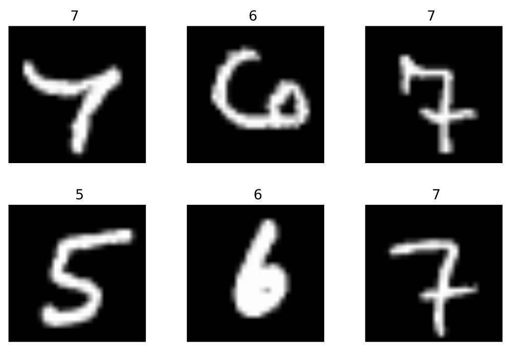
network.eval() # set to evaluation mode

4. Loop over the test images and targets, normalizing and converting each image to a PyTorch tensor, and using the model to predict the corresponding label. Then, resize and display the image with the predicted label as the window name.

# loop over test images
for test_image, test_target in zip(test_data, test_targets):

    # normalize image and convert to tensor
    inference_image = torch.from_numpy(test_image).float() / 255.0
    inference_image = inference_image.unsqueeze(0).unsqueeze(0)

    # predict
    output = network(inference_image)
    pred = output.argmax(dim=1, keepdim=True)
    prediction = str(pred.item())

    test_image = cv2.resize(test_image, (400, 400))
    cv2.imshow(prediction, test_image)
    key = cv2.waitKey(0)
    if key == ord('q'): # break on q key
        break
 
    cv2.destroyAllWindows()

5. Finally, the shows us the results, and the loop is broken when the 'q' key is pressed.

Although this is a simple example, it is a great starting point for a beginner learning PyTorch. In the next tutorial, we will introduce a PyTorch wrapper to simplify the training process and automate some of the steps we took in this tutorial.

Conclusion: 

In this tutorial, we have learned how to build a simple digit classifier using PyTorch. We started by setting up our environment and loading the dataset. We then defined our model and trained it on the dataset. Finally, we tested the model and made predictions. This tutorial is a great starting point for beginners who want to learn about PyTorch and deep learning.

Thank you for following along with this tutorial. You can find the complete code for this tutorial in my GitHub repository. 

Don't forget to subscribe to my YouTube channel for more tutorials like this. See you in the next tutorial!