I am starting a new tutorial series about Transformers. I'll implement them step-by-step in TensorFlow, explaining all the parts. All created layers will be included in Machine Learning Training Utilities ("mltu" PyPi library), so they can be easily reused in other projects. 

At the end of these tutorials, I'll create practical examples of training and using Transformer in NLP tasks.

In this tutorial, I'll walk through the steps to implement the Transformer model from "Attention is All You Need" paper for the machine translation task. The model is based on the Transformer (self-attention) architecture, an alternative to recurrent neural networks (RNNs). The Transformer model is more straightforward than traditional recurrent neural networks and has achieved state-of-the-art results on machine translation tasks.

Table of content:

• Introduction to Transformer Architecture;
• Implementing positional embedding layer;
• Implementing Attention layers;
• Implementing Encoder and Decoder layers;
• Building the Transformer model;
• Preprocessing data for machine translation task;
• Training and Evaluating the model;
• Run inference on new data with a trained model.

Introduction to Transformer Architecture

CNNs and RNNs vs. Transformers

If you were following my blog, I recently was focused on CNNs and RNNs, but I haven't covered Transformers yet. So, what is the difference between Transformers and RNNs?

1. Convolutional Neural Networks (CNNs) are primarily used for image and video-related tasks. They excel at capturing spatial relationships and extracting features from input data. CNNs consist of convolutional layers, pooling layers, and fully connected layers. Convolutional layers use filters to scan and convolve the input data, capturing local patterns and features. Pooling layers shrink the size of the data while keeping the most essential details intact. Fully connected layers provide the final classification or regression outputs.
2. Recurrent Neural Networks (RNNs) are designed for sequential data, such as text or time series. They process input data sequentially, maintaining hidden states that retain information from previous inputs.
   RNNs are like a brain that remembers past information, which makes them useful for tasks where understanding context is essential, like language processing, understanding speech, and translating languages. However, RNNs suffer from vanishing or exploding gradient problems, limiting their ability to capture long-term dependencies.
3. Transformers are a relatively new architecture that gained significant popularity, especially in the field of NLP. Vaswani et al. introduced them in the paper "Attention Is All You Need" in 2017. Transformers rely on self-attention mechanisms to capture global dependencies between input elements. They can process inputs in parallel, making them highly parallelizable and efficient for training on modern hardware. Transformers have achieved state-of-the-art results in various NLP tasks, including language translation, text summarization, and sentiment analysis.

Compared to CNNs and RNNs, Transformers have several advantages:

• Parallelization: Transformers can process input elements in parallel, making them faster to train and more efficient on hardware that supports parallel operations;
• Attention mechanism: Transformers use self-attention to capture global dependencies in the input sequence, allowing them to attend to relevant context across the entire sequence. This is particularly useful in NLP tasks where long-range dependencies are essential.
• No sequential processing: Unlike RNNs, Transformers do not process input sequentially. They can take advantage of parallel processing and are not limited by the sequential nature of RNNs, enabling faster training and inference.

However, Transformers also have some limitations. They typically require large amounts of data to train effectively and can be computationally expensive, especially for longer sequences. Additionally, CNNs and RNNs still perform well for specific tasks, especially when the input data has a grid-like structure (CNNs) or requires sequential processing (RNNs).

In summary, while CNNs and RNNs have their strengths in image and sequential data, respectively, Transformers have emerged as powerful models for NLP tasks, leveraging parallel processing and attention mechanisms to capture global dependencies. The choice of architecture depends on the specific task and characteristics of the input data.

Main components of Transformer architecture

Here is the architecture of the Transformer model with short descriptions of each component:

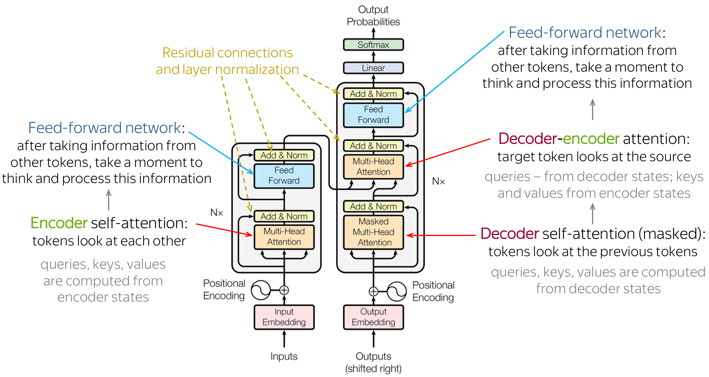
The Transformer architecture is made up of two main parts: the encoder and the decoder. These parts have several layers that use attention and self-attention methods to handle input and output sequences. The encoder changes the input sequence into a hidden representation, and the decoder creates the output sequence using the encoder's hidden representation. The Transformer achieves excellent performance on various language processing tasks by combining these two components. Here are a few notes:

• In more detail, the encoder takes the input sequence and converts it into a series of embeddings. These embeddings are then processed through a stack of identical layers in the encoder. Each layer consists of two sublayers: a self-attention layer and a feedforward layer. The self-attention layer helps the encoder focus on different parts of the input sequence and understand long-range relationships. In contrast, the feedforward layer applies a nonlinear transformation to the hidden representation;
• Similarly, the decoder also has a stack of identical layers. However, each layer in the decoder has three sublayers: a self-attention layer, an encoder-decoder attention layer, and a feedforward layer. The self-attention layer helps the decoder attend to different parts of the output sequence. In contrast, the encoder-decoder attention layer lets the decoder consider different parts of the input sequence;
• Attention is a mechanism that allows the model to concentrate on specific input aspects when making predictions selectively. In the Transformer architecture, attention is used in both the encoder and decoder. It calculates a weighted sum of the input sequence values, where the similarity between the query and the keys determines the weights. This mechanism enables the model to concentrate on various segments of the input sequence depending on the particular task;
• The self-attention mechanism is a specific type of attention used in the Transformer architecture. It operates on the input sequence and transforms it into query, key, and value vectors. The query vectors determine the attention weights for each position in the input sequence based on their similarity to the key vectors. The value vectors are then multiplied by the attention weights and summed up to create a weighted representation of the input sequence. This representation becomes the input for the next layer, enabling the model to attend to different parts of the sequence and capture long-range dependencies.

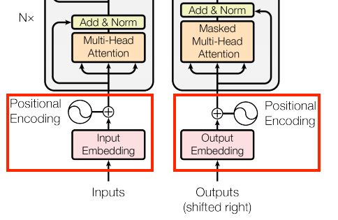
From the above image, you may notice that there is a Positional encoding block added right to the input embeddings. Positional encoding is applied to account for the lack of a recurrence or convolutional structure in the Transformer. It encodes the position of tokens in the input sequence. Each token's embedding is augmented with positional encoding to provide the model with positional information. The positional encoding is calculated using a fixed function that considers the token's position in the sequence and the embedding's dimension. By incorporating this positional information, the model can differentiate between tokens appearing at different positions in the input sequence.

In the official TensorFlow transformer tutorial, we can find this great visualization of how the Encoder and Decoder work while processing input data:

Implementing PositionalEmbedding layers

Positional encoding (positional_encoding function)

In Transformer models, the encoder and decoder components employ a common approach to convert input tokens into vectors:

This is achieved using a "tf.keras.layers.Embedding" layer, which generates a vector representation for each token in the input sequence.

The positional encoding function in the transformers architecture introduces the concept of order or position into the input data. Transformers are designed to process input data in parallel, making them highly efficient for tasks like natural language processing. However, since transformers do not have an inherent sense of order, they cannot naturally capture the sequential or positional information present in the input data.

In applications like language processing, the order of words in a sentence is crucial for understanding the meaning. The positional encoding function is introduced to incorporate this positional information into the model.

The positional encoding function maps each position (or time step) in the input sequence to a vector representation. These positional embeddings are added element-wise to the input embeddings (usually word embeddings) before feeding them into the transformer model. This addition allows the model to distinguish between words based on their positions, enabling it to understand the sequential structure of the input.

The most common type of positional encoding used is based on the sine and cosine functions. This method ensures that the positional embeddings have a consistent pattern, allowing the model to generalize well to longer sequences it might not have seen during training.

In summary, the purpose of the positional encoding function in transformers is to introduce position information into the model, enabling it to understand the sequential nature of the input data and effectively perform tasks where the order of elements matters, such as language translation or language understanding tasks.

The following formula gives the method to compute the positional encoding:

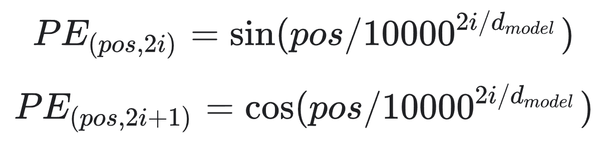
Where "pos" is the position and "i" is the dimension. "d_model" is the dimension of the embedding vector. In other words, each dimension of the positional encoding corresponds to a sinusoid. The position determines the wavelength of each sinusoid, and the dimension determines the frequency. The positional encoding is calculated using sine and cosine functions with different frequencies. The frequencies form a geometric progression from "2/pi" to "10000*2/pi".

Let's implement this layer in the code:

import numpy as np
import tensorflow as tf

for gpu in tf.config.experimental.list_physical_devices('GPU'):
    tf.config.experimental.set_memory_growth(gpu, True)

def positional_encoding(length: int, depth: int):
    """
    Generates a positional encoding for a given length and depth.

    Args:
        length (int): The length of the input sequence.
        depth (int): The depth that represents the dimensionality of the encoding.

    Returns:
        tf.Tensor: The positional encoding of shape (length, depth).
    """
    depth = depth / 2

    positions = np.arange(length)[:, np.newaxis]     # (seq, 1)
    depths = np.arange(depth)[np.newaxis, :]/depth   # (1, depth)

    angle_rates = 1 / (10000**depths)         # (1, depth)
    angle_rads = positions * angle_rates      # (pos, depth)

    pos_encoding = np.concatenate([np.sin(angle_rads), np.cos(angle_rads)], axis=-1) 

    return tf.cast(pos_encoding, dtype=tf.float32)

The positional_encoding function generates a matrix of position encodings to provide information about the position of each token in the input sequence. This helps the self-attention mechanism in the transformer model to differentiate between different token positions.

The function takes two arguments: length, which specifies the size of the input sequence, and depth, which determines the dimensionality of the encoding.

To begin, the function creates two matrices: positions and depths. The positions matrix has a shape of (length, 1) and contains the indices representing the positions in the input sequence. The depths matrix has a shape of (1, depth/2) and contains values ranging from 0 to (depth/2)-1, which are then normalized by dividing them by depth/2.

Next, the function calculates the angle rates using the formula 1 / (10000**depths), resulting in a matrix with a shape of (1, depth/2). These angle rates are used to compute the angle radians by multiplying positions with the angle rates. The resulting matrix has a (length, depth/2) shape.

Finally, the function combines the sine and cosine values of the angle radians along the last axis to create the position encoding matrix. This matrix has a shape of (length, depth). It is then converted to the data type tf.float32 and returned as the final result.

In summary, the positional encoding function employs a set of sine and cosine waves that oscillate at different frequencies, depending on their position within the embedding vector's depth. These oscillations manifest along the position axis. Let's create a visualization to illustrate this concept:

import matplotlib.pyplot as plt

pos_encoding = positional_encoding(length=2048, depth=512)

# Check the shape.
print(pos_encoding.shape)

# Plot the dimensions.
plt.pcolormesh(pos_encoding.numpy().T, cmap='RdBu')
plt.ylabel('Depth')
plt.xlabel('Position')
plt.colorbar()
plt.show()

At the output, we'll see a shape of (2024, 512), and the following image:

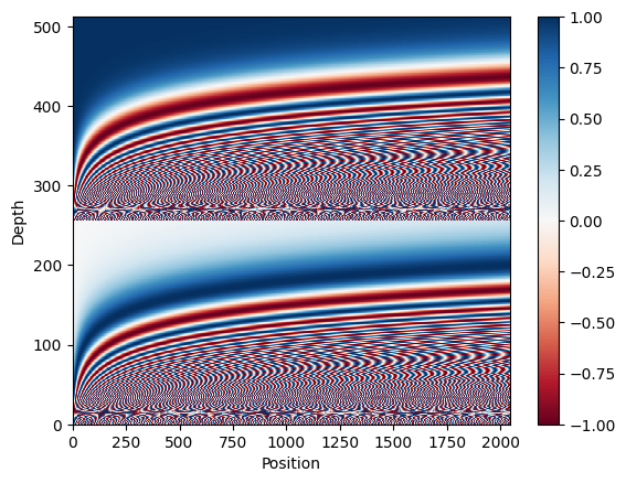
This visualization aims to help us understand the positional encoding matrix and observe how it varies across different positions and depths in the sequence. It also ensures that the encoding values are appropriately normalized and distributed throughout the matrix.

To provide a visual representation, we will plot the cosine similarity between the positional encoding vector at index 1000 and all the other vectors in the positional encoding matrix.

Before calculating the cosine similarity, the positional encoding vectors undergo L2 normalization. Then, using the einsum function, the code computes the dot product between the positional encoding vector at index 1000 and each vector in the matrix. The resulting dot products are displayed in a graph, where the y-axis represents the cosine similarity values between the vectors:

pos_encoding /= tf.norm(pos_encoding, axis=1, keepdims=True)
p = pos_encoding[1000]
dots = tf.einsum('pd,d->p', pos_encoding, p).numpy()

plt.subplot(2, 1, 1)
plt.plot(dots)
plt.ylim([0, 1])
plt.plot([950, 950, float('nan'), 1050, 1050], [0, 1, float('nan'), 0, 1], color='k', label='Zoom')
plt.legend()

plt.subplot(2, 1, 2)
plt.plot(range(len(dots)), dots)
plt.xlim([950, 1050])
plt.ylim([0, 1])

After running the above code, we would see the following image:

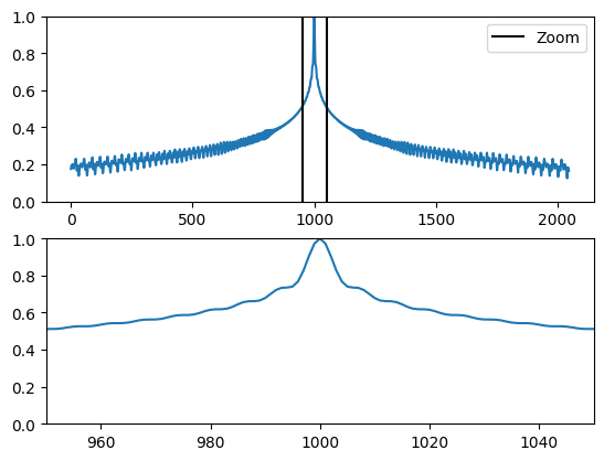
The visualization consists of two plots. The first plot displays the entire cosine similarity graph, while the second plot zooms in on a specific range of values between index 950 and 1050.

This visualization aims to demonstrate how the positional encoding vectors capture the position information of each token in the sequence. When the cosine similarity values are high between vectors, it suggests that they are positioned closely along the position axis. This indicates that these vectors share similar positional information, emphasizing the importance of positional encoding in preserving the order of tokens within the sequence.

PositionalEmbedding layer

Now that we know how to implement positional encoding, we can create a custom layer that will combine positional encoding with token embedding. This layer will be used in Encoder and Decoder layers:

class PositionalEmbedding(tf.keras.layers.Layer):
    """
    A positional embedding layer combines the input embedding with a positional encoding that helps the Transformer
    to understand the relative position of the input tokens. This layer takes the input of tokens and converts them
    into sequence of embeddings vector. Then, it adds the positional encoding to the embeddings.

    Methods:
        compute_mask: Computes the mask to be applied to the embeddings.
        call: Performs the forward pass of the layer.
    """
    def __init__(self, vocab_size: int, d_model: int, embedding: tf.keras.layers.Embedding=None):
        """ Constructor of the PositionalEmbedding layer.

        Args:
            vocab_size (int): The size of the vocabulary. I. e. the number of unique tokens in the input sequence.
            d_model (int): The dimensionality of the embedding vector.
            embedding (tf.keras.layers.Embedding): The custom embedding layer. If None, a default embedding layer will be created.
        """
        super().__init__()
        self.d_model = d_model
        self.embedding = tf.keras.layers.Embedding(vocab_size, d_model, mask_zero=True) if embedding is None else embedding
        self.pos_encoding = positional_encoding(length=2048, depth=d_model)

    def compute_mask(self, *args, **kwargs):
        """ Computes the mask to be applied to the embeddings.
        """
        return self.embedding.compute_mask(*args, **kwargs)

    def call(self, x: tf.Tensor) -> tf.Tensor:
        """ Performs the forward pass of the layer.
        
        Args:
            x (tf.Tensor): The input tensor of shape (batch_size, seq_length).

        Returns:
            tf.Tensor: The output sequence of embedding vectors with added positional information. The shape is
                (batch_size, seq_length, d_model).
        """
        x = self.embedding(x)
        length = tf.shape(x)[1]
        # This factor sets the relative scale of the embedding and positonal_encoding.
        x *= tf.math.sqrt(tf.cast(self.d_model, tf.float32))
        x = x + self.pos_encoding[tf.newaxis, :length, :]
        return x

Above, we created a PositionalEmbedding layer that combines an embedding layer and a positional encoding function. The class takes two arguments: vocab_size, which is the size of the vocabulary of the input sequences, and d_model, which is the size of the embedding and positional encoding vectors. This layer aims to encode input sequences in a transformer model by adding positional information to the token embeddings.

In the constructor of this class, two crucial components are created. An Embedding layer is established to convert input tokens into embedding vectors. Secondly, a positional encoding matrix is generated using the positional_encoding function, having a shape of (max_length, d_model).

This class compute_mask method produces a mask that matches the shape of the input tensor destined for the embedding layer.

In the call method, the input tensor undergoes a few main steps:

1. It is passed through the embedding layer to obtain the embedding output;
2. The result is scaled by the square root of the d_model value;
3. The positional encoding matrix is added to the embedding output corresponding to each input token;
4. The encoded input sequence is returned as the final output.

In most cases, when constructing a Transformer model, we would create two separate positional embedding layers for the encoder and decoder components. Because the encoder and decoder have different input sequences, they require different positional encoding matrices. However, in this tutorial, we'll test the output of this layer by creating a single positional embedding layer, and as an input, we'll use random sequences of integers:

vocab_size = 1000
d_model = 512

embedding_layer = PositionalEmbedding(vocab_size, d_model)

random_input = np.random.randint(0, vocab_size, size=(1, 100))

output = embedding_layer(random_input)
print("random_input shape", random_input.shape)
print("PositionalEmbedding output", output.shape)

In the terminal, we should see the following:

random_input shape (1, 100)
PositionalEmbedding output (1, 100, 512)

As we can see, we created a random input tensor of shape (1, 100) and passed it through the PositionalEmbedding layer. The output of this layer has the shape of (1, 100, 512), where 100 is the length of the input sequence, and 512 is the dimensionality of the embedding and positional encoding vectors.

A vector of size 512 represents each token in the input sequence. The positional encoding vectors are added to the embedding vectors, providing information about the position of each token in the sequence. This allows the model to understand the order of tokens in the input sequence.

Conclusion:

In this tutorial, we embarked on a comprehensive journey into the fascinating world of Transformers, a revolutionary architecture that has become a game-changer in natural language processing. The step-by-step implementation in TensorFlow and detailed explanations of each component gave readers a deep understanding of how Transformers work.

A notable highlight of the tutorial is the emphasis on reusability and collaboration. By incorporating all created layers into the "mltu" PyPi library, the tutorial encourages knowledge-sharing and facilitates easy integration of these components into other projects.

The comparison of Transformers with traditional CNNs and RNNs highlighted the advantages of Transformers, especially in parallelization and capturing long-range dependencies. While Transformers excel in NLP tasks, the tutorial acknowledged their limitations, making it a well-rounded and balanced architecture exploration.

There will be a series of tutorials until we can construct a final trainable Transformer model. But I encourage you to spend time in all these tutorials to understand the components of a Transformer. Later, it will be easier to adapt this architecture to different tasks; I am talking from my experience. So, don't stop your journey here; move on to the next tutorial!