In the previous tutorials, I covered the whole architecture of the transformer model in TensorFlow. We implemented all the necessary layers to construct and compile the Transformer model that we could use for any sequence-to-sequence task. Although in this tutorial, I demonstrated how to prepare and preprocess your data efficiently to use it in the training process. So, this is a continuation tutorial from the previous parts to demonstrate how to combine everything and finally train your model!

If you want to avoid reading everything step-by-step, jump straight to my GitHub code. I'll walk through this code step by step.

The Transformer model has proven highly effective in various natural language processing tasks, including machine translation.

We start by importing the necessary libraries and modules. But before that, we need to download a dataset that we'll use for training. I chose to use the Opus100 Spanish-to-English translation dataset for this task. But to simplify the problem, not to download this dataset manually, I wrote a Python script to do so. The following code is in the download.py file:

import os
import requests
from tqdm import tqdm
from bs4 import BeautifulSoup

# URL to the directory containing the files to be downloaded
language = "en-es"
url = f"https://data.statmt.org/opus-100-corpus/v1.0/supervised/{language}/"
save_directory = f"./Datasets/{language}"

# Create the save directory if it doesn't exist
os.makedirs(save_directory, exist_ok=True)

# Send a GET request to the URL
response = requests.get(url)

# Parse the HTML response
soup = BeautifulSoup(response.content, 'html.parser')

# Find all the anchor tags in the HTML
links = soup.find_all('a')

# Extract the href attribute from each anchor tag
file_links = [link['href'] for link in links if '.' in link['href']]

# Download each file
for file_link in tqdm(file_links):
    file_url = url + file_link
    save_path = os.path.join(save_directory, file_link)
    
    print(f"Downloading {file_url}")
    
    # Send a GET request for the file
    file_response = requests.get(file_url)
    if file_response.status_code == 404:
        print(f"Could not download {file_url}")
        continue
    
    # Save the file to the specified directory
    with open(save_path, 'wb') as file:
        file.write(file_response.content)
    
    print(f"Saved {file_link}")

print("All files have been downloaded.")

The above code will create a folder Datasets/en-es/ where it will put all the downloaded files. Before running this, you will need to install the beautifulsoup4 library.

After this, we have our dataset files ready and can move on to the training script.

Main requirements for this tutorial:

• mltu==1.1.0
• tensorflow>=2.10
• tf2onnx==1.14.0 (to convert the trained model to onnx format)
• onnx==1.12.0 (to convert the trained model to onnx format)

Step 1: Importing Libraries and Setting up GPU Memory Growth:

So, let's import stuff that we'll be using:

import numpy as np

import tensorflow as tf
try: [tf.config.experimental.set_memory_growth(gpu, True) for gpu in tf.config.experimental.list_physical_devices("GPU")]
except: pass

from keras.callbacks import EarlyStopping, ModelCheckpoint, ReduceLROnPlateau, TensorBoard
from mltu.tensorflow.callbacks import Model2onnx, WarmupCosineDecay

from mltu.tensorflow.dataProvider import DataProvider
from mltu.tokenizers import CustomTokenizer

from mltu.tensorflow.transformer.utils import MaskedAccuracy, MaskedLoss
from mltu.tensorflow.transformer.callbacks import EncDecSplitCallback

Now, let's create another file model.py and write the following code that we'll use to construct our Transformer model in TensorFlow:

#model.py
import tensorflow as tf

from mltu.tensorflow.transformer.layers import Encoder, Decoder

def Transformer(
    input_vocab_size: int, 
    target_vocab_size: int, 
    encoder_input_size: int = None,
    decoder_input_size: int = None,
    num_layers: int=6, 
    d_model: int=512, 
    num_heads: int=8,
    dff: int=2048,
    dropout_rate: float=0.1,
    ) -> tf.keras.Model:
    """
    A custom TensorFlow model that implements the Transformer architecture.

    Args:
        input_vocab_size (int): The size of the input vocabulary.
        target_vocab_size (int): The size of the target vocabulary.
        encoder_input_size (int): The size of the encoder input sequence.
        decoder_input_size (int): The size of the decoder input sequence.
        num_layers (int): The number of layers in the encoder and decoder.
        d_model (int): The dimensionality of the model.
        num_heads (int): The number of heads in the multi-head attention layer.
        dff (int): The dimensionality of the feed-forward layer.
        dropout_rate (float): The dropout rate.

    Returns:
        A TensorFlow Keras model.
    """
    inputs = [
        tf.keras.layers.Input(shape=(encoder_input_size,), dtype=tf.int64), 
        tf.keras.layers.Input(shape=(decoder_input_size,), dtype=tf.int64)
        ]
    
    encoder_input, decoder_input = inputs

    encoder = Encoder(num_layers=num_layers, d_model=d_model, num_heads=num_heads, dff=dff, vocab_size=input_vocab_size, dropout_rate=dropout_rate)(encoder_input)
    decoder = Decoder(num_layers=num_layers, d_model=d_model, num_heads=num_heads, dff=dff, vocab_size=target_vocab_size, dropout_rate=dropout_rate)(decoder_input, encoder)

    output = tf.keras.layers.Dense(target_vocab_size)(decoder)

    return tf.keras.Model(inputs=inputs, outputs=output)

As you might see, we need to set many arguments while creating a Transformer model, but you should already be familiar with them from my previous tutorial; I covered them in detail. To control these arguments and others while training a Transformer model, creating a configuration file that we could change in one place is a good idea. To do so, create a configs.py file with the following configuration code:

#configs.py
import os
from datetime import datetime

from mltu.configs import BaseModelConfigs


class ModelConfigs(BaseModelConfigs):
    def __init__(self):
        super().__init__()
        self.model_path = os.path.join(
            "Models/09_translation_transformer",
            datetime.strftime(datetime.now(), "%Y%m%d%H%M"),
        )
        self.num_layers = 4
        self.d_model = 128
        self.num_heads = 8
        self.dff = 512
        self.dropout_rate = 0.1
        self.batch_size = 16
        self.train_epochs = 50
        # CustomSchedule parameters
        self.init_lr = 0.00001
        self.lr_after_warmup = 0.0005
        self.final_lr = 0.0001
        self.warmup_epochs = 2
        self.decay_epochs = 18

Here, we can define our Transformer size by changing num_layers, d_model, num_heads, dff, and dropout_rate. Also, we can set training parameters for the training loop, learning rate, etc. While following this tutorial, you'll understand what is used to what.

Let's return back to our main train.py code and import our model and configurations. Also, we'll create an object for our defined configurations that will be held there:

#train.py
from model import Transformer
from configs import ModelConfigs

configs = ModelConfigs()

Step 2: Define and Load Dataset Paths:

Next, we need to define the paths to the training and validation dataset for both English and Spanish languages:

# Path to dataset
en_training_data_path = "Datasets/en-es/opus.en-es-train.en"
en_validation_data_path = "Datasets/en-es/opus.en-es-dev.en"
es_training_data_path = "Datasets/en-es/opus.en-es-train.es"
es_validation_data_path = "Datasets/en-es/opus.en-es-dev.es"

Step 3: Read and Prepare Dataset:

Now, we must read and prepare the training and validation datasets for both languages and filter out sentences longer than the specified maximum length. This ensures that the model is manageable for the model:

def read_files(path):
    with open(path, "r", encoding="utf-8") as f:
        en_train_dataset = f.read().split("\n")[:-1]
    return en_train_dataset

en_training_data = read_files(en_training_data_path)
en_validation_data = read_files(en_validation_data_path)
es_training_data = read_files(es_training_data_path)
es_validation_data = read_files(es_validation_data_path)

# Consider only sentences with length <= 500
max_lenght = 500
train_dataset = [[es_sentence, en_sentence] for es_sentence, en_sentence in zip(es_training_data, en_training_data) if len(es_sentence) <= max_lenght and len(en_sentence) <= max_lenght]
val_dataset = [[es_sentence, en_sentence] for es_sentence, en_sentence in zip(es_validation_data, en_validation_data) if len(es_sentence) <= max_lenght and len(en_sentence) <= max_lenght]
es_training_data, en_training_data = zip(*train_dataset)
es_validation_data, en_validation_data = zip(*val_dataset)

Step 4: Tokenization:

Now, we need to create tokenizers for both Spanish and English languages. To do so, we'll use the CustomTokenizer class. Tokenization involves converting sentences into sequences of integers, which the model can process. The fit_on_texts method is used to fit the tokenizers on the training data:

# prepare spanish tokenizer, this is the input language
tokenizer = CustomTokenizer(char_level=True)
tokenizer.fit_on_texts(es_training_data)
tokenizer.save(configs.model_path + "/tokenizer.json")

# prepare english tokenizer, this is the output language
detokenizer = CustomTokenizer(char_level=True)
detokenizer.fit_on_texts(en_training_data)
detokenizer.save(configs.model_path + "/detokenizer.json")

Step 5: Data Preprocessing Function:

def preprocess_inputs(data_batch, label_batch):
    encoder_input = np.zeros((len(data_batch), tokenizer.max_length)).astype(np.int64)
    decoder_input = np.zeros((len(label_batch), detokenizer.max_length)).astype(np.int64)
    decoder_output = np.zeros((len(label_batch), detokenizer.max_length)).astype(np.int64)

    data_batch_tokens = tokenizer.texts_to_sequences(data_batch)
    label_batch_tokens = detokenizer.texts_to_sequences(label_batch)

    for index, (data, label) in enumerate(zip(data_batch_tokens, label_batch_tokens)):
        encoder_input[index][:len(data)] = data
        decoder_input[index][:len(label)-1] = label[:-1] # Drop the [END] tokens
        decoder_output[index][:len(label)-1] = label[1:] # Drop the [START] tokens

    return (encoder_input, decoder_input), decoder_output

This function preprocesses the input data and labels for the model. It converts sentences into integer sequences using the tokenizers and prepares the input-output pairs for Transformer training. More details about this step can be found in my previous tutorial.

Step 6: Create Data Providers:

# Create Training Data Provider
train_dataProvider = DataProvider(
    train_dataset, 
    batch_size=configs.batch_size, 
    batch_postprocessors=[preprocess_inputs],
    use_cache=True,
    )

# Create Validation Data Provider
val_dataProvider = DataProvider(
    val_dataset, 
    batch_size=configs.batch_size, 
    batch_postprocessors=[preprocess_inputs],
    use_cache=True,
    )

We create data providers for training and validation using the DataProvider class. Data providers are responsible for feeding data to the model during training. Here, we can control the batch size we use for training (decrease for lower GPU memory usage) and integrate data preprocessing.

Step 7: Define the Transformer Model:

# Create TensorFlow Transformer Model
transformer = Transformer(
    num_layers=configs.num_layers,
    d_model=configs.d_model,
    num_heads=configs.num_heads,
    dff=configs.dff,
    input_vocab_size=len(tokenizer)+1,
    target_vocab_size=len(detokenizer)+1,
    dropout_rate=configs.dropout_rate,
    encoder_input_size=tokenizer.max_length,
    decoder_input_size=detokenizer.max_length
    )

transformer.summary()

Here, we create an instance of the Transformer model using the Transformer class from the previously created model.py script. We specify the model's architecture, including the number of layers, model dimensions, number of heads, and more. But I prefer changing these settings so we can later save these settings with the model, and we'll know what configurations we used to train our Transformer model.

At the output, we should see the following transformer model summary:

__________________________________________________________________________________________________
 Layer (type)                   Output Shape         Param #     Connected to
==================================================================================================
 input_1 (InputLayer)           [(None, 502)]        0           []

 input_2 (InputLayer)           [(None, 502)]        0           []

 encoder (Encoder)              (None, 502, 128)     2738688     ['input_1[0][0]']

 decoder (Decoder)              (None, 502, 128)     4884864     ['input_2[0][0]',
                                                                  'encoder[0][0]']

 dense_16 (Dense)               (None, 502, 1055)    136095      ['decoder[0][0]']

==================================================================================================
Total params: 7,759,647
Trainable params: 7,759,647
Non-trainable params: 0
__________________________________________________________________________________________________

Step 8: Compile the Model:

optimizer = tf.keras.optimizers.Adam(learning_rate=configs.init_lr, beta_1=0.9, beta_2=0.98, epsilon=1e-9)

# Compile the model
transformer.compile(
    loss=MaskedLoss(),
    optimizer=optimizer,
    metrics=[MaskedAccuracy()],
    run_eagerly=False
    )

We compile the model by specifying the loss function, optimizer, and metrics for evaluation. The MaskedLoss and MaskedAccuracy functions are custom components designed to handle masking in sequence-to-sequence tasks, such as machine translation, where sequences of variable lengths are processed in batches. Masking is necessary to ignore padding tokens during the computation of loss and accuracy.

Here's an explanation of what these components are and why they are used:

• MaskedLoss - In sequence-to-sequence tasks like machine translation, sequences often have varying lengths. To efficiently process batches of sequences, sequences are padded with special tokens (usually "padding" or "mask" tokens) to match the length of the most extended sequence in the batch. However, these padding tokens should not contribute to the loss computation when calculating loss, as they don't represent actual data.
  When computing the loss, the MaskedLoss function is a custom loss function that applies masking to ignore the padding tokens. It calculates the loss by considering only the non-padding tokens in the target sequences. This ensures that the model's predictions are compared only with the actual tokens in the target sequences.
• MaskedAccuracy - Similar to the MaskedLoss, the MaskedAccuracy function is a custom accuracy metric that takes into account the masking of padding tokens. Only the non-padding tokens in the target sequences are considered when computing accuracy. This ensures that the accuracy is calculated based on the relevant tokens the model predicts.

In both cases, these custom functions help ensure that the model's performance metrics (loss and accuracy) are accurately calculated without being influenced by the padding tokens, which are used for sequence alignment in batch processing.

Step 9: Define Callbacks:

In this step, we define various callbacks that control the training process. These callbacks provide functionalities like learning rate scheduling, early stopping, model checkpointing, and more. The specific callbacks used here are instances of classes provided by the custom mltu library:

# Define callbacks
warmupCosineDecay = WarmupCosineDecay(
    lr_after_warmup=configs.lr_after_warmup,
    final_lr=configs.final_lr,
    warmup_epochs=configs.warmup_epochs,
    decay_epochs=configs.decay_epochs,
    initial_lr=configs.init_lr,
    )
earlystopper = EarlyStopping(monitor="val_masked_accuracy", patience=5, verbose=1, mode="max")
checkpoint = ModelCheckpoint(f"{configs.model_path}/model.h5", monitor="val_masked_accuracy", verbose=1, save_best_only=True, mode="max", save_weights_only=False)
tb_callback = TensorBoard(f"{configs.model_path}/logs")
reduceLROnPlat = ReduceLROnPlateau(monitor="val_masked_accuracy", factor=0.9, min_delta=1e-10, patience=2, verbose=1, mode="max")
model2onnx = Model2onnx(f"{configs.model_path}/model.h5", metadata={"tokenizer": tokenizer.dict(), "detokenizer": detokenizer.dict()}, save_on_epoch_end=False)
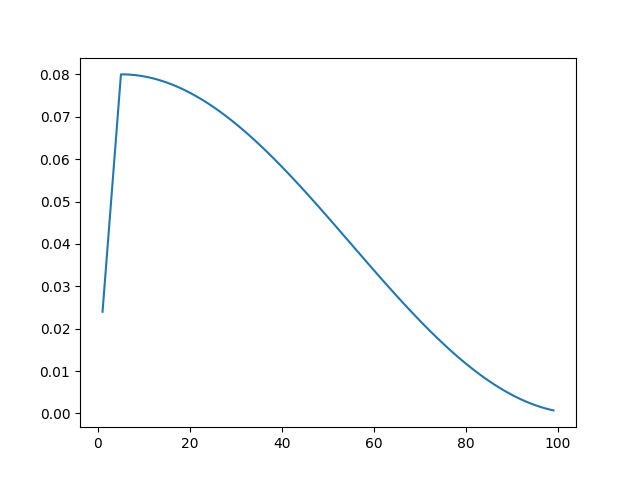
encDecSplitCallback = EncDecSplitCallback(configs.model_path, encoder_metadata={"tokenizer": tokenizer.dict()}, decoder_metadata={"detokenizer": detokenizer.dict()})

We define the most popular callbacks, so we won't need to track, save, or, in other ways, manually modify the training process. These callbacks will handle all training. Let's take a look at the WarmupCosineDecay callback. That's a learning rate scheduler that combines two common techniques: warm-up and cosine annealing, which are often used to control the learning rate during the training process of neural networks. It's a way to dynamically adjust the learning rate over time to improve training stability and convergence. Let's dive into the details of how it works:

Warm-up: During the initial stages of training, especially in the early epochs, using a high learning rate can cause the optimization process to become unstable or result in extensive weight updates that lead to overshooting. Warm-up involves gradually increasing the learning rate from a small value to its desired value over a few initial epochs. This allows the model to start with minor weight updates and gradually increase the learning rate as the optimization process stabilizes.

Cosine Annealing: Cosine annealing is a learning rate schedule that reduces the learning rate smoothly and periodically. It's called "cosine annealing" because the learning rate follows a cosine curve pattern. This approach helps the model converge more effectively and escape local minima in the loss landscape. The learning rate decreases during each period, and after each period, it restarts from its maximum value.

The WarmupCosineDecay function combines these two techniques to provide a well-balanced learning rate schedule. Here's how it works:

1. Warm-up Phase: During the warm-up phase, the learning rate gradually increases from an initial value (initial_lr) to a specified learning rate after warm-up (lr_after_warmup) over a certain number of epochs (warmup_epochs).

2. Cosine Annealing Phase: After the warm-up phase, the learning rate starts to follow a cosine annealing pattern. The learning rate varies in a cosine manner between the lr_after_warmup and a lower value (final_lr) over the course of decay_epochs epochs.

The combination of warm-up and cosine annealing helps to mitigate the challenges of both early instabilities due to high learning rates and the later convergence slowdown due to a decreasing learning rate. This dynamic learning rate schedule often results in more stable training and better convergence properties.

Here is an example representing the change in learning rate during training:

We'll talk about EncDecSplitCallback in the next tutorial, where we'll check the trained Transformer model and try to run the translation.

Step 10: Transformer training:

Finally, we train the Transformer model using the fit method. We provide the training and validation data providers along with the defined callbacks to monitor and control the training process:

# Train the model
transformer.fit(
    train_dataProvider, 
    validation_data=val_dataProvider, 
    epochs=configs.train_epochs,
    callbacks=[
        warmupCosineDecay,
        checkpoint, 
        tb_callback, 
        reduceLROnPlat,
        model2onnx,
        encDecSplitCallback
        ]
    )

Conclusion:

Congratulations! We have successfully created a Spanish-to-English translation Transformer model using TensorFlow. In this tutorial, we covered various aspects of the process, including data preprocessing, model architecture, compilation, and training. You can further customize and enhance the model by experimenting with different hyperparameters and training strategies.

Remember that NLP models can be resource-intensive and might require significant computational resources, especially for large datasets. Ensure you have access to a GPU or other high-performance hardware for efficient training.

Feel free to modify and extend this tutorial according to your specific needs and further explore the capabilities of the Transformer architecture in machine translation tasks. Happy coding!

See you in the next tutorial, where I'll demonstrate how to use this model in production to translate Spanish to English language!

The complete code for this tutorial you can find in this GitHub link.

The trained model and results can be downloaded from here.