Deep Neural Networks step by step initialize

Welcome to another tutorial. In the last tutorial series, we wrote 2 layers neural networks model. Now it's time to build a deep neural network, where we could have whatever count of layers we want.

So the same as in previous tutorials, we'll first implement all the functions required to build a deep neural network. Then we will use these functions to build a deep neural network for image classification (cats vs. dogs).

In this tutorial series, I will use non-linear units like ReLU to improve our model. Our deep neural network model will be built to easily define deep layers that our model would be easy to use.

This is a continuation tutorial of my one hidden layer neural network tutorial to use the same data set. If you see this tutorial first time, cats vs. dogs data-set you can get from my GitHub page. If you don't know how to use a data set, check my previous tutorials.

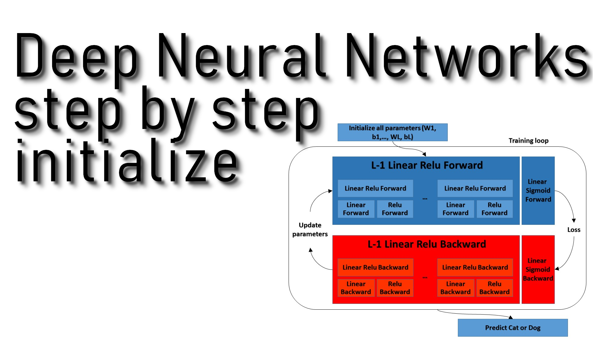
First, let's define our model structure:

Same as in previous tutorials, build a deep neural network and implement several "helper functions". These helper functions will be used to build a two-layer neural network and an L-layer neural network. In each small helper function, we will implement, I will try to give you a detailed explanation. So what we'll do in this tutorial series:

• Initialize the parameters for a two-layer network and an L-layer neural network;
• Implement the forward propagation module (shown in the figure below);
  - Complete the LINEAR part of a layer's forward propagation step (resulting in Z[l]);
  - We'll write the ACTIVATION function (relu/sigmoid);
  - We'll combine the previous two steps into a new [LINEAR->ACTIVATION] forward function;
  - Stack the [LINEAR->RELU] forward function L-1 time (for layers 1 through L-1) and add a [LINEAR->SIGMOID] at the end (for the final layer L). This will give us a new L_model_forward function;
• Compute the loss;
• Implement the backward propagation module (denoted in red in the figure below);
  - Complete the LINEAR part of a layer's backward propagation step;
  - We will write the gradient of the ACTIVATE function (relu_backward/sigmoid_backward);
  - Combine the previous two steps into a new [LINEAR->ACTIVATION] backward function;
  - Stack [LINEAR->RELU] backward L-1 times and add [LINEAR->SIGMOID] backward in a new L_model_backward function;
• Finally, update the parameters.

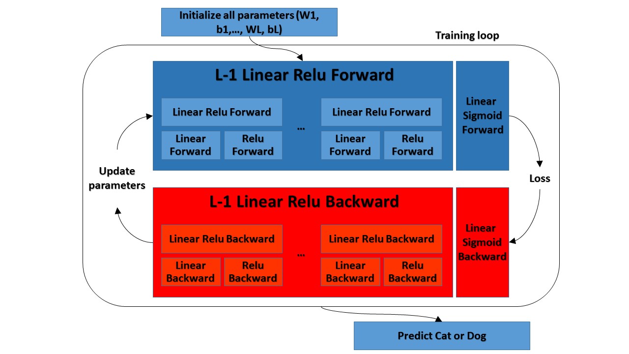You will see that for every forward function; there will be a corresponding backward function. That is why we will be storing some values in a cache at every step of our forward module. The cached values will be useful for computing gradients. In the backpropagation module, we will then use the cache to calculate the gradients. In this tutorial series, I will show you exactly how to carry out each of these steps.

Parameters initialization:

I will write two helper functions that will initialize the parameters for our model. The first function will be used to initialize parameters for a two-layer model. The second one will generalize this initialization process to L layers.

So not to write my code twice, I will copy my initialization function for a two-layer model from my previous tutorial:

def initialize_parameters(input_layer, hidden_layer, output_layer):
    # initialize 1st layer output and input with random values
    W1 = np.random.randn(hidden_layer, input_layer) * 0.01
    # initialize 1st layer output bias
    b1 = np.zeros((hidden_layer, 1))
    # initialize 2nd layer output and input with random values
    W2 = np.random.randn(output_layer, hidden_layer) * 0.01
    # initialize 2nd layer output bias
    b2 = np.zeros((output_layer,1))
    
    parameters = {"W1": W1,
                  "b1": b1,
                  "W2": W2,
                  "b2": b2}
    
    return parameters

Parameters initialization for a deeper L-layer neural network is more complicated because there are many more weight matrices and bias vectors. When we complete our initialize_parameters_deep function, we should make sure that our dimensions match each layer.

Recall that n[l] is the number of units in layer l. Thus, for example, if the size of our input X is (12288,6002) (with m=6002 examples), then:

I should remind you that when we compute WX+b in python, it carries out broadcasting. For example, if:

Then WX+b will be:

So what we'll do to implement the initialization function for an L-layer Neural Network:

• The model's structure will be: *[LINEAR -> RELU] × (L-1) -> LINEAR -> SIGMOID*. In our example, it will have L−1 layers using a ReLU activation function followed by an output layer with a sigmoid activation function;
• We'll use random initialization for the weight matrices: np.random.randn(shape)∗0.01;
• We'll use zeros initialization for the biases. Use np.zeros(shape);
• We will store n[l], the number of units in different layers, in a variable 'layer_dims'. For example, if we declare 'layer_dims' to be [2,4,1]: There will be two inputs, one hidden layer with 4 hidden units and an output layer with 1 output unit. This means W1's shape was (4,2), b1 was (4,1), W2 was (1,4), and b2 was (1,1). Now we will generalize this to L layers.

Before moving further, we need to overview the whole notation:

• Superscript [l] denotes a quantity associated with the lth layer. For example, a[L] is the Lth layer activation. W[L] and b[L] are the Lth layer parameters;
• Superscript (i) denotes a quantity associated with the ith example. Example: x(i) is the ith training example;
• Lowerscript i denotes the ith entry of a vector. Example: a[i] denotes the ith entry of the lth layer's activations.

Code for our deep parameters initialization:

Arguments:

layer_dimensions - python array (list) containing the dimensions of each layer in our network

Return:

• parameters - python dictionary containing our parameters "W1", "b1", ..., "WL", "bL":
  Wl - weight matrix of shape (layer_dimensions[l], layer_dimensions[l-1]);
  bl - bias vector of shape (layer_dimensions[l], 1).

def initialize_parameters_deep(layer_dimensions):  
    parameters = {}
    
    # number of layers in the network
    L = len(layer_dimensions) 

    for l in range(1, L):
        parameters['W' + str(l)] = np.random.randn(layer_dimensions[l], layer_dimensions[l-1]) * 0.01
        parameters['b' + str(l)] = np.zeros((layer_dimensions[l], 1))
        
    return parameters

So we wrote our function. Let's test it out with random numbers:

parameters = initialize_parameters_deep([4,5,3])
print("W1 = ", parameters["W1"])
print("b1 = ", parameters["b1"])
print("W2 = ", parameters["W2"])
print("b2 = ", parameters["b2"])

We'll receive:

W1 =  [[ 0.00415369 -0.00965885  0.0009098  -0.00426353]
 [-0.00807062  0.01026888  0.00625363  0.0035793 ]
 [ 0.00829245 -0.00353761  0.00454806 -0.00741405]
 [ 0.00433758 -0.01485895  0.00437019 -0.00712647]
 [ 0.00103969 -0.00245844  0.02399076 -0.02490289]]
b1 =  [[0.]
 [0.]
 [0.]
 [0.]
 [0.]]
W2 =  [[-0.00999478 -0.01071253 -0.00471277  0.01213727 -0.00630878]
 [-0.005903    0.00163863 -0.0143418   0.00660419  0.00885867]
 [ 0.00554906 -0.00170923 -0.00708474 -0.0086883   0.00935947]]
b2 =  [[0.]
 [0.]
 [0.]]

You may receive different values because of random initialization. Let's test deeper initialization:

parameters = initialize_parameters_deep([4,5,3,2])
print("W1 = ", parameters["W1"])
print("b1 = ", parameters["b1"])
print("W2 = ", parameters["W2"])
print("b2 = ", parameters["b2"])
print("W3 = ", parameters["W3"])
print("b3 = ", parameters["b3"])

Then we'll receive something to this:

W1 =  [[-0.00787148  0.00351103  0.00031584  0.01036506]
 [-0.01367634 -0.00592318 -0.01703005 -0.0008115 ]
 [ 0.00681571  0.00115347 -0.00538494  0.00715979]
 [-0.01463998  0.00024354 -0.00847364  0.01652647]
 [-0.00830651  0.0013722   0.01029079 -0.00819454]]
b1 =  [[0.]
 [0.]
 [0.]
 [0.]
 [0.]]
W2 =  [[-0.00646581  0.00884422  0.00472376  0.01447212 -0.00341151]
 [ 0.00102133 -0.00362436 -0.00198458 -0.01005361 -0.00591243]
 [ 0.02244886  0.00919089  0.00110354  0.00086251  0.01074991]]
b2 =  [[0.]
 [0.]
 [0.]]
W3 =  [[-0.00515514 -0.01256405  0.00632316]
 [-0.00304877 -0.00194744  0.00062086]]
b3 =  [[0.]
 [0.]]

Full tutorial code:

import numpy as np

def initialize_parameters(input_layer, hidden_layer, output_layer):
    # initialize 1st layer output and input with random values
    W1 = np.random.randn(hidden_layer, input_layer) * 0.01
    # initialize 1st layer output bias
    b1 = np.zeros((hidden_layer, 1))
    # initialize 2nd layer output and input with random values
    W2 = np.random.randn(output_layer, hidden_layer) * 0.01
    # initialize 2nd layer output bias
    b2 = np.zeros((output_layer,1))
    
    parameters = {"W1": W1,
                  "b1": b1,
                  "W2": W2,
                  "b2": b2}
    
    return parameters

def initialize_parameters_deep(layer_dimensions):  
    parameters = {}
    
    # number of layers in the network
    L = len(layer_dimensions) 

    for l in range(1, L):
        parameters['W' + str(l)] = np.random.randn(layer_dimensions[l], layer_dimensions[l-1]) * 0.01
        parameters['b' + str(l)] = np.zeros((layer_dimensions[l], 1))
        
    return parameters

parameters = initialize_parameters_deep([4,5,3])
print("W1 = ", parameters["W1"])
print("b1 = ", parameters["b1"])
print("W2 = ", parameters["W2"])
print("b2 = ", parameters["b2"])