Deep Neural Networks Final Predict Model

Deep Neural Network for Image Classification:

This tutorial will use the functions we had implemented in the previous parts to build a Deep Neural Network and apply it to cat vs. dog classification. Hopefully, we will see an improvement in accuracy relative to our previous logistic regression implementation. After this part, we will build and apply a Deep Neural Network to supervised learning using only the NumPy library.

Let's first import all the packages that we will need during this part. We will use the same "Cat vs. Dog" dataset as in the Logistic Regression as a Neural Network tutorial. The model we had built had 60% test accuracy on classifying cats vs. dogs images. Hopefully, our new model will perform better!

I'll import code we already wrote from the "Logistic Regression" tutorial series:

import os
import cv2
import numpy as np
import matplotlib.pyplot as plt
import sklearn
from sklearn import datasets

ROWS = 64
COLS = 64
CHANNELS = 3

def read_image(file_path):
    img = cv2.imread(file_path, cv2.IMREAD_COLOR)
    return cv2.resize(img, (ROWS, COLS), interpolation=cv2.INTER_CUBIC)

def prepare_data(images):
    m = len(images)
    X = np.zeros((m, ROWS, COLS, CHANNELS), dtype=np.uint8)
    y = np.zeros((1, m))
    for i, image_file in enumerate(images):
        X[i,:] = read_image(image_file)
        if 'dog' in image_file.lower():
            y[0, i] = 1
        elif 'cat' in image_file.lower():
            y[0, i] = 0
    return X, y

TRAIN_DIR = 'Train_data/'
TEST_DIR = 'Test_data/'

train_images = [TRAIN_DIR+i for i in os.listdir(TRAIN_DIR)]
test_images =  [TEST_DIR+i for i in os.listdir(TEST_DIR)]

train_set_x, train_set_y = prepare_data(train_images)
test_set_x, test_set_y = prepare_data(test_images)

train_set_x_flatten = train_set_x.reshape(train_set_x.shape[0], ROWS*COLS*CHANNELS).T
test_set_x_flatten = test_set_x.reshape(test_set_x.shape[0], -1).T

train_set_x = train_set_x_flatten/255
test_set_x = test_set_x_flatten/255

L-layer deep neural network:

It is hard to represent a deep neural network with a figure. However, here is a simplified network representation:

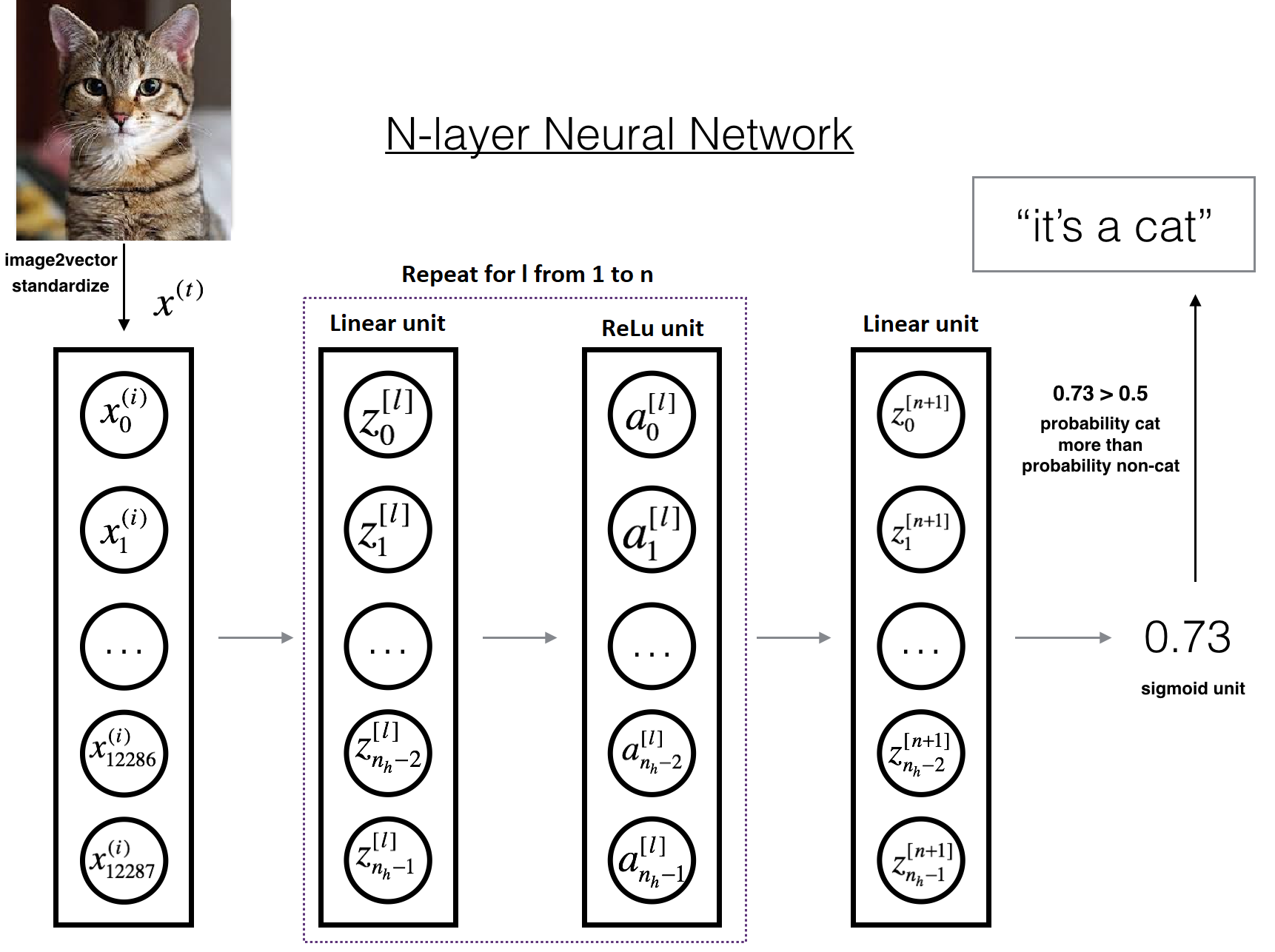
The model can be summarized as: [LINEAR -> RELU] × (L-1) -> LINEAR -> SIGMOID. Detailed Architecture of above figure:

• The input is a (64,64,3) image that is flattened to a vector of size (12288,1);
• The corresponding vector: ${[x_0, x_1, ..., x_{12287}]}^T$ is then multiplied by the weight matrix W^[1], and then you add the intercept b^[1]. The result is called the linear unit;
• Next, you take the ReLu of the linear unit. This process could be repeated several times for each (W[l], b[l]) depending on the model architecture;
• Finally, you take the sigmoid of the final linear unit. If it is greater than 0.5, you classify it to be a cat.

General methodology:

As usual, we will follow the Deep Learning methodology to build the model:

1. Initialize parameters / Define hyperparameters.
2. Loop for num_iterations:

• Forward propagation;
• Compute cost function;
• Backward propagation;
• Update parameters (using parameters and grads from backprop).

3. Use trained parameters to predict labels.

L-layer Neural Network:

We'll use the helper functions we have implemented previously to build an L-layer neural network with the following structure: [LINEAR -> RELU]×(L-1) -> LINEAR -> SIGMOID.

Arguments:

X - data, NumPy array of shape (number of examples, ROWS * COLS * CHANNELS );
Y - true "label" vector (containing 0 if cat, 1 if dog), of shape (1, number of examples);
layers_dims - a list containing the input size and each layer size, of length (number of layers + 1);
learning_rate - learning rate of the gradient descent update rule;
num_iterations - number of iterations of the optimization loop;
print_cost - if True, it prints the cost every 100 steps.

Return:

Parameters -- parameters learned by the model. They can then be used to predict.

def L_layer_model(X, Y, layers_dims, learning_rate = 0.0075, num_iterations = 3000, print_cost=False):#lr was 0.009
    # keep track of cost
    costs = []
    
    # Parameters initialization.
    parameters = initialize_parameters_deep(layers_dims)

    # Loop (gradient descent)
    for i in range(0, num_iterations):

        # Forward propagation: [LINEAR -> RELU]*(L-1) -> LINEAR -> SIGMOID.
        AL, caches = L_model_forward(X, parameters)
        
        # Compute cost.
        cost = compute_cost(AL, Y)
    
        # Backward propagation.
        grads = L_model_backward(AL, Y, caches)
 
        # Update parameters.
        parameters = update_parameters(parameters, grads, learning_rate)
                
        # Print the cost every 100 training example
        if print_cost and i % 100 == 0:
            print ("Cost after iteration %i: %f" %(i, cost))
        if print_cost and i % 100 == 0:
            costs.append(cost)
            
    # plot the cost
    plt.plot(np.squeeze(costs))
    plt.ylabel('cost')
    plt.xlabel('iterations (per tens)')
    plt.title("Learning rate =" + str(learning_rate))
    plt.show()
    
    return parameters

Predict function:

Before training our model, we need to write a predict function that will be used to predict the results of an L-layer neural network:

Arguments:

X - a data set of examples you would like to label.
Parameters - parameters of the trained model.

Return:

p - predictions for the given dataset X.

def predict(X, parameters):
    m = X.shape[1]

    # number of layers in the neural network
    n = len(parameters) // 2
    p = np.zeros((1,m))
    
    # Forward propagation
    probas, caches = L_model_forward(X, parameters)

    # convert probas to 0/1 predictions
    for i in range(0, probas.shape[1]):
        if probas[0,i] > 0.5:
            p[0,i] = 1
        else:
            p[0,i] = 0   
        
    return p

We are now ready to train our deep neural networks model. So we can run the cell below to train our model. The cost should decrease on every iteration. In my case, with 6000 images, it may take more than a day on my CPU to run 10000 iterations. Here is the code:

layers_dims = [12288, 800, 10, 1] #  4-layer model
parameters = L_layer_model(train_set_x, train_set_y, layers_dims, learning_rate = 0.1, num_iterations = 10000, print_cost = True)

print("train accuracy: {} %".format(100 - np.mean(np.abs(predict(train_set_x, parameters) - train_set_y)) * 100))
print("test accuracy: {} %".format(100 - np.mean(np.abs(predict(test_set_x, parameters) - test_set_y)) * 100))

My updated Cat vs. Dog training results:

Cost after iteration 9600: 0.409001
Cost after iteration 9700: 0.468013
Cost after iteration 9800: 0.464725
Cost after iteration 9900: 0.440395
train accuracy: 75.50816394535155 %
test accuracy: 63.9 %

And here is the training cost plot:

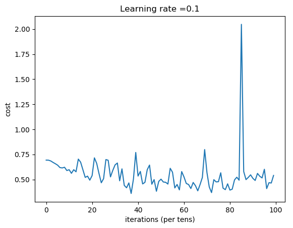
From our test accuracy, you can see that it's almost not better in classifying cats versus dogs. It's because simple neural networks can't do it very well. We need to use Convolutional Neural Networks to get better results (using them in future tutorials).

We will test our deep neural network code with the below code. So there are two functions: to create data, which we will use to train our model. Another function will be used to plot decision boundary in our plot, which was predicted by our neural network; not getting deeper into these functions, here they are:

def load_dataset(DataNoise = 0.05, Visualize = False):
    #np.random.seed(1)
    train_X, train_Y = sklearn.datasets.make_circles(n_samples=300, noise=DataNoise)
    #np.random.seed(2)
    test_X, test_Y = sklearn.datasets.make_circles(n_samples=100, noise=DataNoise)
    train_X = train_X.T
    train_Y = train_Y.reshape((1, train_Y.shape[0]))
    test_X = test_X.T
    test_Y = test_Y.reshape((1, test_Y.shape[0]))
    # Visualize the data
    if Visualize == True:
        axes = plt.gca()
        axes.set_xlim([-1.5,1.5])
        axes.set_ylim([-1.5,1.5])
        plt.scatter(train_X[0, :], train_X[1, :], c=train_Y[0], s=40, cmap=plt.cm.Spectral)
        plt.show()

    return train_X, train_Y, test_X, test_Y

def plot_decision_boundary(model, X, y):
    # Set min and max values and give it some padding
    x_min, x_max = X[0, :].min() - 1, X[0, :].max() + 1
    y_min, y_max = X[1, :].min() - 1, X[1, :].max() + 1
    h = 0.01
    
    # Generate a grid of points with distance h between them
    xx, yy = np.meshgrid(np.arange(x_min, x_max, h), np.arange(y_min, y_max, h))
    
    # Predict the function value for the whole grid
    Z = model(np.c_[xx.ravel(), yy.ravel()])
    Z = Z.reshape(xx.shape)
    
    # Plot the contour and training examples
    plt.contourf(xx, yy, Z, cmap=plt.cm.Spectral)
    plt.ylabel('x2')
    plt.xlabel('x1')
    axes = plt.gca()
    axes.set_xlim([-1.5,1.5])
    axes.set_ylim([-1.5,1.5])
    plt.scatter(X[0, :], X[1, :], c=y[0], cmap=plt.cm.Spectral)
    plt.show()

Let's visualize our training data with the following line:

train_X, train_Y, test_X, test_Y = load_dataset(DataNoise = 0.15, Visualize = True)

Let's plot our training data:

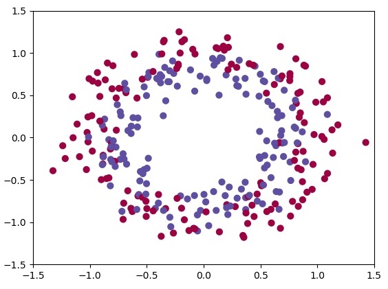
At first, we'll try to use a neural network with one hidden layer, where input is 2, 4 hidden layers and output equal to 1:

layers_dims = [2, 4, 1]
parameters = L_layer_model(train_X, train_Y, layers_dims, learning_rate = 0.2, num_iterations = 15000, print_cost = True)

print("train accuracy: {} %".format(100 - np.mean(np.abs(predict(train_X, parameters) - train_Y)) * 100))
plot_decision_boundary(lambda x: predict(x.T, parameters), train_X, train_Y)

With 15000 iterations and a learning rate of 0.2, we received an accuracy of 61%:

Cost after iteration 14600: 0.654744
Cost after iteration 14700: 0.654740
Cost after iteration 14800: 0.654737
Cost after iteration 14900: 0.654733
train accuracy: 61.333333333333336 %

And here is the classification plot:

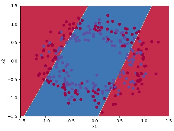
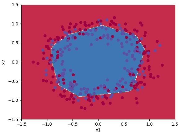
It doesn't look nice so let's try the same 15000 iterations and learning rate of 0.2 with 10 hidden layers:

Cost after iteration 14600: 0.534574
Cost after iteration 14700: 0.534570
Cost after iteration 14800: 0.534569
Cost after iteration 14900: 0.534564
train accuracy: 73.33333333333333 %

Now we received 73% accuracy. That's nice; let's plot our result:

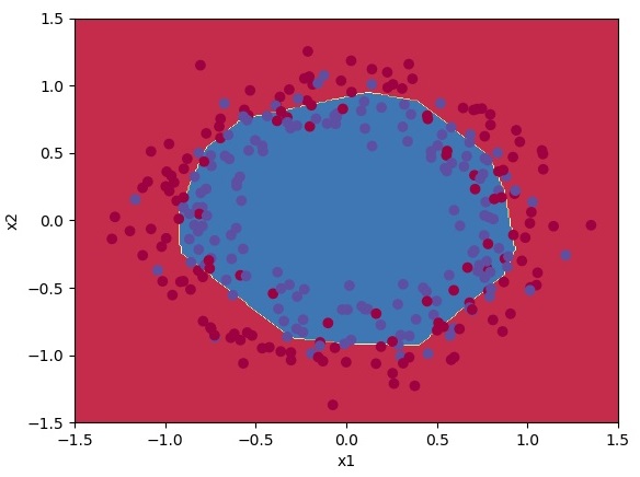
And now, let's test our hard work and try a deeper network with layers_dims = [2, 128, 4, 1].

Cost after iteration 14600: 0.504184
Cost after iteration 14700: 0.504572
Cost after iteration 14800: 0.504701
Cost after iteration 14900: 0.504019
train accuracy: 74.33333333333334 %

Now we received 74% accuracy. That's nice, but as you can see, it's getting harder to get better results. Let's plot our result:

Conclusion: