In a previous tutorial, I introduced you to the Yolo v3 algorithm background, network structure, feature extraction, and finally, we made a simple detection with original weights. In this part, I’ll cover the Yolo v3 loss function and model training. We’ll train a custom object detector on the Mnist dataset.

Loss function

In YOLO v3, the author regards the target detection task as the regression problem of target area prediction and category prediction, so its loss function is somewhat different. For the loss function, Redmon J did not explain in detail in the Yolo v3 paper. But I found Yolo loss explanation in this link; the loss function looks following:

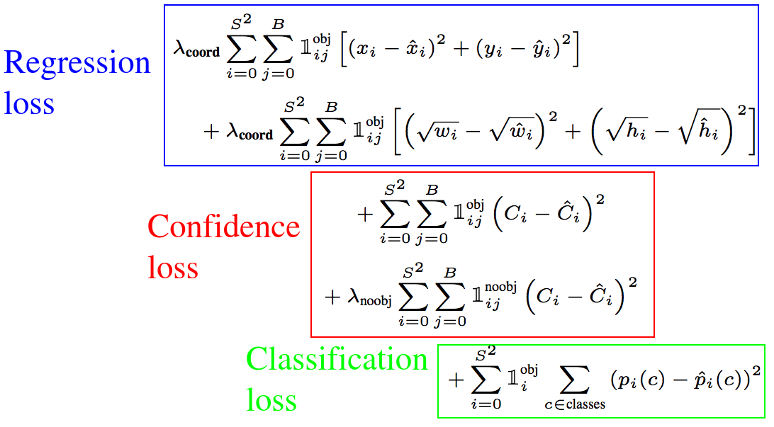However, through the interpretation of the darknet source code, the loss function of YOLO v3 can be summarized as follows:

• Confidence loss, determine whether there are objects in the prediction frame;
• Box regression loss, calculated only when the prediction box contains objects;
• Classification loss, decide which category the things in the prediction frame belong to.

Loss of confidence

YOLO v3 directly optimizes the confidence loss to let the model learn to distinguish the background and foreground areas of the picture, which is similar to the RPN function in Faster R-CNN:

The rule of determination is simple: if the IoU of a prediction box and all actual boxes is less than a certain threshold, it is determined to be the background. Otherwise, it is the foreground (including objects).

Classification loss

The classification loss used here is the cross-entropy of the two classifications. The classification problem of all categories is reduced to whether it belongs to this category so that multi-classification is regarded as a two-classification problem. The advantage of this is to exclude the mutual exclusion of the classes, especially to solve the problem of missed detection due to the overlapping of multiple categories of objects.

$Loss=\frac{-1}{n}\sum _x(y*\ln (a)+(1-y)*\ln (1-a\left)\right)$

This looks as follows:

respond_bbox = label[:,:,:,:, 4:5] 
prob_loss = respond_bbox * tf.nn.sigmoid_cross_entropy_with_logits (labels = label_prob, logits = conv_raw_prob

Box regression loss

Box regression loss in code looks as follows:

respond_bbox  = label[:, :, :, :, 4:5]
bbox_loss_scale = 2.0 - 1.0 * label_xywh[:, :, :, :, 2:3] * label_xywh[:, :, :, :, 3:4] / (input_size ** 2)
giou_loss = respond_bbox * bbox_loss_scale * (1 - giou)
giou_loss = tf.reduce_mean(tf.reduce_sum(giou_loss, axis=[1,2,3,4]))

• The smaller the size of the bounding box, the larger the value of bbox_loss_scale. We know that the anchors in YOLO v1 have done root and width processing in the Loss, which is to weaken the impact of the size of the bounding box on the loss value;
• Respond_bbox means that if the grid cell contains objects, then the bounding box loss will be calculated;
• The larger the value of GIoU between the two bounding boxes, the smaller the loss value of GIoU, so the network will optimize towards the direction of higher overlap between the prediction box and the actual box.

In my implementation, the original IoU loss was replaced with GIoU loss. This improved the detection accuracy by about 1%. The advantage of GIoU is that it enhances the distance measurement method between the prediction box and the anchor box.

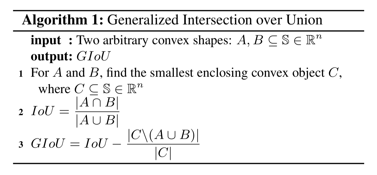
GIoU background introduction

This is quite a new proposed way to optimize the bounding box-GIoU (Generalized IoU). The bounding box is generally represented by the coordinates of the upper left corner and the lower right corner, namely (x1, y1, x2, y2). Well, you find that this is a vector. The L1 norm or L2 norm can generally measure the distance of the vector. However, the detection effect is very different when the L1 and L2 norms take the same value. The direct performance is that the IoU value of the prediction and the actual detection frame changes significantly, which shows that the L1 and L2 norms are not very good to Reflect the detection effect.

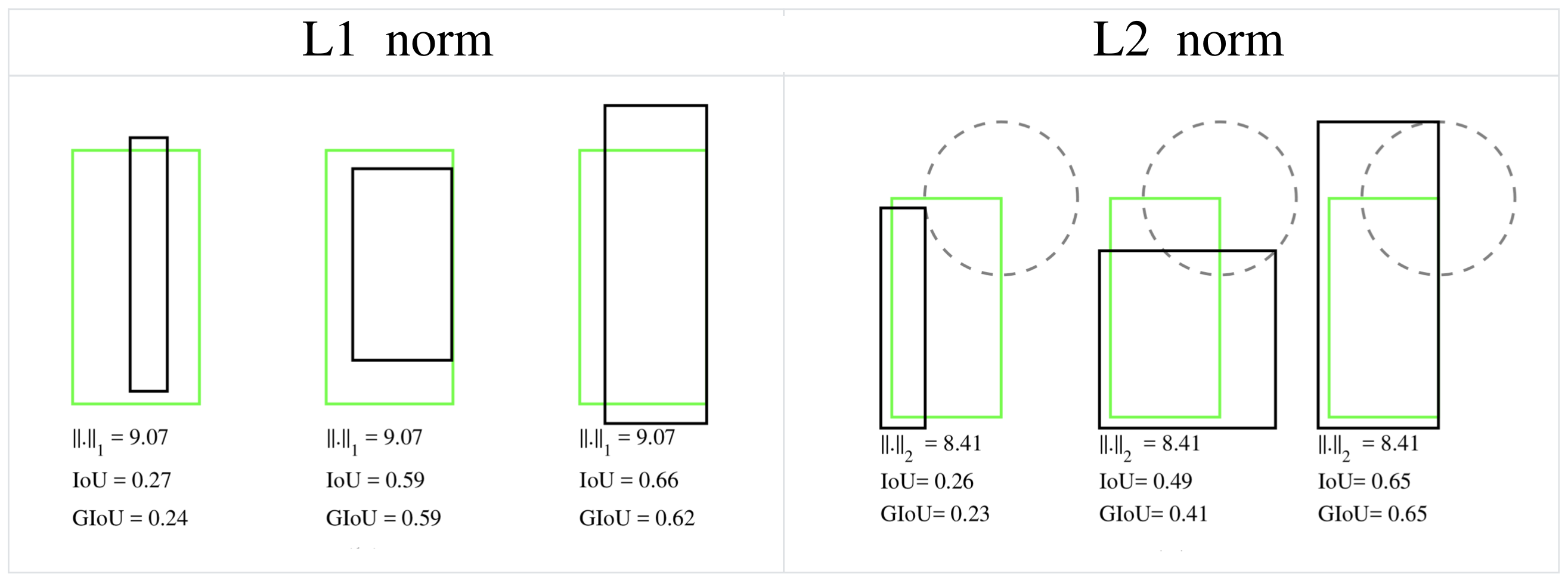When the L1 or L2 norms are the same, it is found that the values of IoU and GIoU are very different, which indicates that it is not appropriate to use the L norm to measure the distance of the bounding box. In this case, the academic community generally uses the IoU to calculate the similarity between two bounding boxes. The author found that using IoU has two disadvantages, making it less suitable for loss function:

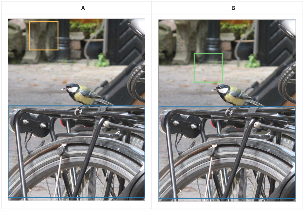
• When there is no coincidence between the prediction box and the actual box, the IoU value is 0, which results in a gradient of 0 when optimizing the loss function, which means that it cannot be optimized. For example, the IoU value of scene A and scene B are both 0, but the prediction effect of scene B is better than A because the distance between the two bounding boxes is closer (the L norm is smaller):
  
• Even when the prediction box and the actual box coincide and have the same IoU value, the detection effect has a significant difference, as shown in the following figure:
  

The three images above have IoU = 0.33, but the GIoU values are 0.33, 0.24, and -0.1, respectively. This indicates that the better the two bounding boxes overlap and align, the higher the GIOU value will be.

GIoU calculation formula:

And here how it looks in code (part from original code):

def bbox_giou (boxes1, boxes2):
    ...
    # Calculate the iou value between the two bounding boxes     
    iou = inter_area / union_area 
    
    # Calculate the coordinates of the upper left corner and the lower right corner of the smallest closed convex surface     
    enclose_left_up = tf.minimum (boxes1 [..., :2], boxes2 [..., :2])    
    enclose_right_down = tf.maximum (boxes1 [..., 2:], boxes2 [..., 2:])    
    enclose = tf.maximum(enclose_right_down-enclose_left_up, 0.0 ) 
    
    # Calculate the area of the smallest closed convex surface C     
    enclose_area = enclose [..., 0 ] * enclose [..., 1 ] 

    # Calculate the GIoU value according to the GioU formula     
    giou = iou- 1.0 * (enclose_area-union_area) / enclose_area 

    return giou

Model training

Weight initialization

One problem training neural networks faces, especially Deep Neural Networks, is that the gradient disappears or the gradient explodes. This means that when we train a Deep Network, the derivative or slope sometimes becomes very large, very small, or even decreases exponentially. At this time, the Loss we see will become NaN. Suppose we are training such an extremely Deep Neural Network. The activation function g(z)=z is used for simplicity, and the bias parameter is ignored.

First, we assume that g(z)=z, b[l]=0, so for the target output:

$\text{If} W^{\left[l\right]}=\left[\begin{array}{cccc}1.5& 0& 0& 1.5\end{array}\right], \text{then} \hat{y}=W^{\left[L\right]}{\left[\begin{array}{cc}1.5& 0\\ 0& 1.5\end{array}\right]}^{[L-1]}X, \text{the value of the activation function will increase exponentially;}$

$\text{If} W^{\left[l\right]}=\left[\begin{array}{cccc}0.5& 0& 0& 0.5\end{array}\right], \text{then} \hat{y}=W^{\left[L\right]}{\left[\begin{array}{cc}0.5& 0\\ 0& 0.5\end{array}\right]}^{[L-1]}X, \text{the value of the activation function will decrease exponentially;}$

The intuitive understanding here is: if the weight W is only slightly larger than one or the unit matrix, the output of the deep neural network will explode. And if W is somewhat smaller than 1, it may be 0.9; the output value of each layer of the network will decrease exponentially. This means that the proper weight value initialization is particularly important! The following is a simple code to show this:

import numpy as np
import tensorflow as tf
import matplotlib.pyplot as plt
%matplotlib inline
plt.figure(figsize=(20,10))

x = np.random.randn(2000, 800) * 0.01 # Create input data
stds = [0.25, 0.2, 0.15, 0.1, 0.05, 0.04, 0.03, 0.02] # Try to use different standard deviations so that the initial weights are different

for i, std in enumerate(stds):
    # First layer - fully connected layer
    dense_1 = tf.keras.layers.Dense(750, kernel_initializer=tf.random_normal_initializer(stddev=std), activation='tanh')
    output_1 = dense_1(x)
    # Second layer - fully connected layer
    dense_2 = tf.keras.layers.Dense(700, kernel_initializer=tf.random_normal_initializer(stddev=std), activation='tanh')
    output_2 = dense_2(output_1)
    # Third layer - fully connected layer
    dense_3 = tf.keras.layers.Dense(650, kernel_initializer=tf.random_normal_initializer(stddev=std), activation='tanh')
    output_3 = dense_3(output_2).numpy().flatten()

    plt.subplot(1, len(stds), i+1)
    plt.hist(output_3, bins=600, range=[-1, 1])
    plt.xlabel('std = %.3f' %std)
    plt.yticks([])
plt.show()

After running this above code, you should see the following chart:

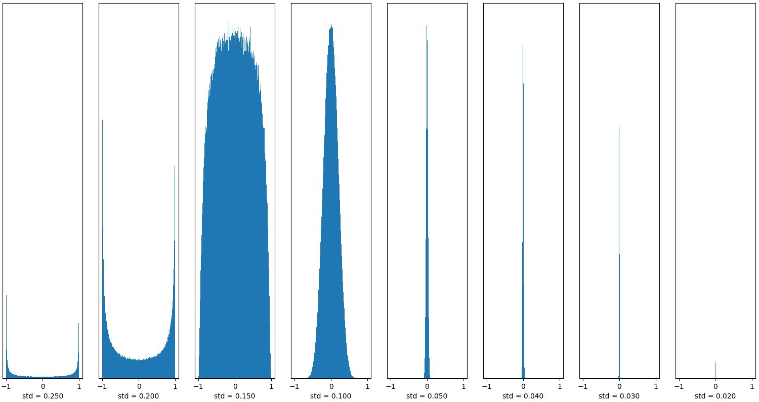We can see that when the standard deviation is large (std => 0.25), almost all output values are concentrated near -1 or 1, which indicates that the Neural Network has a gradient explosion at this time. When the standard deviation is small (std = 0.03 and 0.02), we see that the output value is quickly approaching 0, which indicates that the gradient of the neural network has disappeared at this time. If the standard deviation of the initialization weight is too large or too small, NaN may appear while training the network.

Learning rate

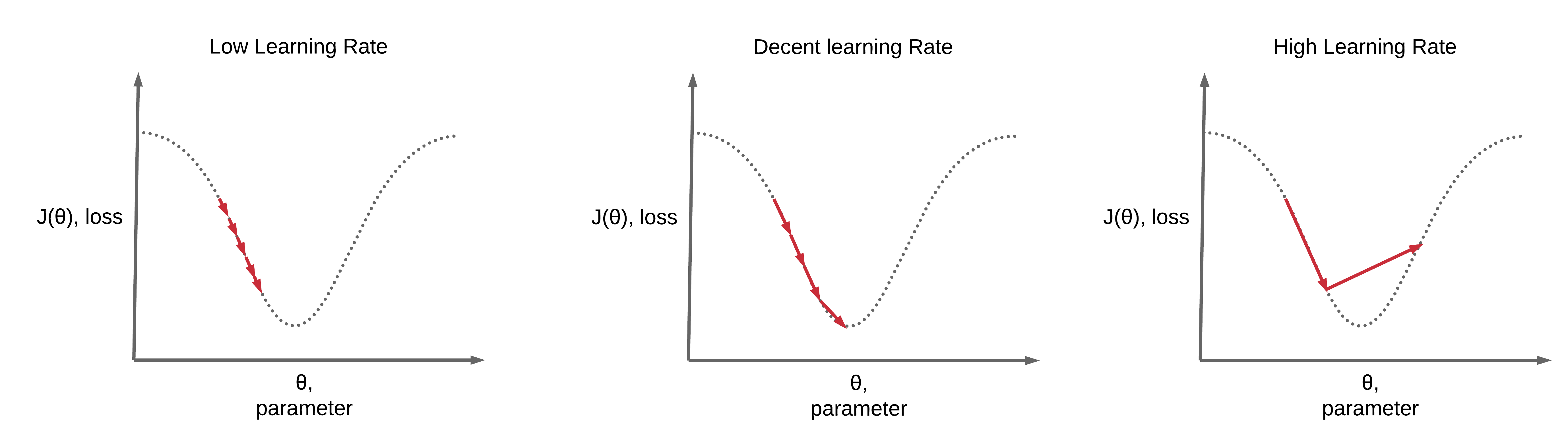
The learning rate is one of the hyperparameters that the most affect performance. If we can only adjust one hyperparameter, then the best choice is the learning rate. In most cases, the improper selection of learning rate causes Loss to become NaN. The following image shows that gradient descent can be slow if the learning rate is too low. If the learning rate is too large, gradient descent can overshoot the minimum. It may fail to converge or even diverge.

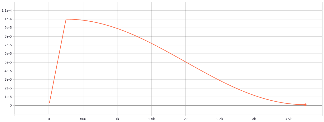
Since the Neural Network is very unstable at the beginning of training, the learning rate should be set very low to ensure that the network can have good convergence. But the lower learning rate will make the training process very slow, so here we will use a way to gradually increase the lower learning rate to a higher learning rate to achieve the “warmup” stage of network training, called the warmup stage. About warmup, you can read on this paper.

But suppose we minimize the Loss of Network training. In that case, it is not appropriate to always use a higher learning rate because it will make the weight gradient oscillate back and forth, and it is difficult to make the Loss of training reach the global minimum. Therefore, the cosine attenuation method in the same paper is adopted in the end. This stage can be called a consensus decay stage. This is how our learning rate chart will look like:

Pre-trained Yolo v3 model weights

The current mainstream approach to target detection is to extract features based on the pre-trained model of the Imagenet dataset and then perform fine-tuning training on target detection (such as the YOLO algorithm) on the COCO dataset referred to as transfer learning. Transfer learning is based on a similar distribution of the data set. For example, the Mnist is entirely different from the COCO dataset distribution. There is no need to load the COCO pre-training model.

Quick training for custom Mnist dataset

To test if custom Yolo v3 object detection training works for you, you must first complete the tutorial steps to ensure that simple detection with original weights works for you.

When you have cloned the GitHub repository, you should see the “mnist” folder containing mnist images. From these images, we create mnist training data with the following command:

python mnist/make_data.py

This make_data.py script creates training and testing images in the correct format. Also, this makes an annotation file. One line for one image, in the form like the following:

image_absolute_path xmin,ymin,xmax,ymax,label_index xmin2,ymin2,xmax2,ymax2,label_index2 ...

The origin of coordinates is at the left top corner, left top => (xmin, ymin), right bottom => (xmax, ymax), label_index is in range [0, class_num — 1]. We’ll talk more about this in the next tutorial, where I will show you how to train the YOLO model with your custom data.

./yolov3/configs.py file is already configured for Mnist training.

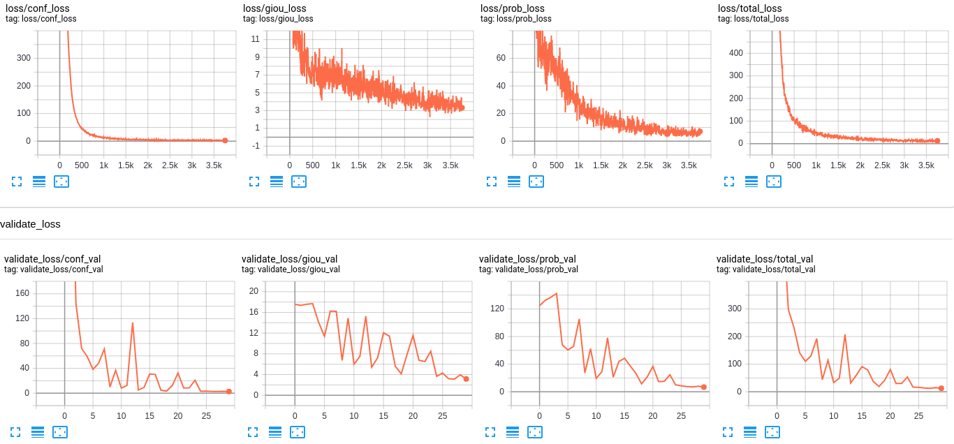
Now, you can train it and then evaluate your model running these commands from a terminal: python train.py tensorboard --logdir ./log

Track your training progress in Tensorboard by going to http://localhost:6006/; after a while, you should see similar results to this:

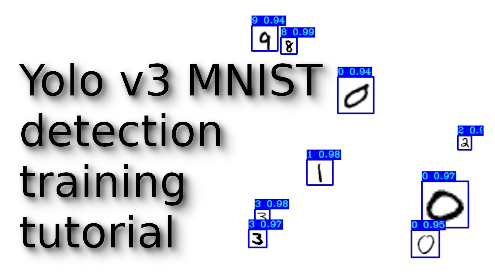
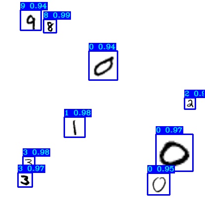
When the training process is finished, you can test detection with detect_mnist.py script: python detect_mnist.py

Then you should see similar results to the following:

Conclusion:

That’s it for this tutorial. We learned how the Loss works in the Yolo v3 algorithm, and we trained our first custom object detector with the Mnist dataset. This was relatively easy because I prepared all files to test training with only a few commands.

In the next part, I will show you how to configure everything for custom objects training, transfer weights from the original weights file, and finally fine-tuning with your classes. See you in the next part!