Hello everyone! I'll introduce you to Generative Adversarial Networks in TensorFlow in this tutorial. To simplify everything, we will use the MNIST digits dataset to generate new digits! First, it is better to start with DCGAN instead of simple GAN. You'll get the results you want faster. The only difference is that DCGAN uses deep Neural Networks instead of simple ones. The Generative Adversarial Networks goal is to generate new data similar to the training data. 

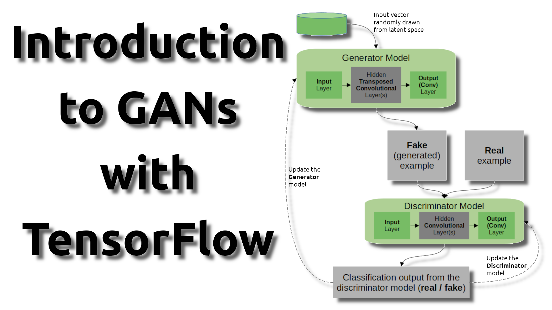
The diagram below illustrates how the two models interact within the GAN architecture.

The dataset used in this tutorial is MNIST -  a collection of 28x28 grayscale images of handwritten digits from 0 to 9. Later, after knowing how everything works, we'll be able to use our GAN model for more challenging tasks.

Here are the steps we will be following in this tutorial:

1. Load and preprocess the MNIST dataset;
2. Define the generator and discriminator models;
3. Define the loss functions for the generator and discriminator;
4. Train the DCGAN model;
5. Generate new MNIST digits using the trained model.

Before we start, ensure you have TensorFlow installed on your machine. You can install it using pip:

pip install tensorflow==2.10.*

1. Load and preprocess the MNIST dataset

First, we need to load the MNIST dataset. TensorFlow provides a convenient way to download and load the dataset:

import tensorflow as tf
from tensorflow.keras.datasets import mnist

# Load MNIST dataset
(x_train, y_train), (x_test, y_test) = mnist.load_data()

# Normalize pixel values to [-1, 1]
x_train = (x_train.astype('float32') - 127.5) / 127.5 

In the code above, we load the MNIST dataset and normalize the pixel values to be between -1 and 1. This is a common preprocessing step for GANs when we use them for images. This is because most of the time, within the Generator network, we use "tanh" activation, which gives us output that ranges from -1 to 1. We may receive similar images when we transform this value back to 0-255. 

2. Define the generator and discriminator models

Next, we need to define the generator and discriminator models. The generator takes a random noise vector as input and generates an image, while the discriminator takes an image as input and outputs a binary classification (real or fake).

import tensorflow as tf
from keras import layers

# Define the generator model
def build_generator(noise_dim):
    inputs = layers.Input(shape=noise_dim, name="input")

    x = layers.Dense(7*7*256, use_bias=False)(inputs)
    x = layers.BatchNormalization()(x)
    x = layers.LeakyReLU()(x)

    x = layers.Reshape((7, 7, 256))(x)
    assert x.shape == (None, 7, 7, 256)  # Note: None is the batch size

    x = layers.Conv2D(128, (5, 5), strides=(1, 1), padding='same', use_bias=False)(x)
    assert x.shape == (None, 7, 7, 128)
    x = layers.BatchNormalization()(x)
    x = layers.LeakyReLU()(x)

    x = layers.UpSampling2D(size=(2, 2))(x)
    x = layers.Conv2D(64, (5, 5), strides=(1, 1), padding='same', use_bias=False)(x)
    assert x.shape == (None, 14, 14, 64)
    x = layers.BatchNormalization()(x)
    x = layers.LeakyReLU()(x)

    x = layers.UpSampling2D(size=(2, 2))(x)
    x = layers.Conv2D(1, (5, 5), strides=(1, 1), padding='same', use_bias=False)(x)

    # add last acvitaion layer of tanh
    x = layers.Activation('tanh')(x)
    assert x.shape == (None, 28, 28, 1)

    model = tf.keras.Model(inputs=inputs, outputs=x)

    return model


# Define the discriminator model
def build_discriminator(img_shape):
    inputs = layers.Input(shape=img_shape, name="input")

    x = layers.Conv2D(64, (5, 5), strides=(2, 2), padding='same')(inputs)
    x = layers.LeakyReLU(0.2)(x)

    x = layers.Conv2D(128, (5, 5), strides=(2, 2), padding='same')(x)
    x = layers.LeakyReLU(0.2)(x)

    x = layers.Flatten()(x)
    x = layers.Dropout(0.3)(x)
    x = layers.Dense(1, activation="sigmoid")(x)

    model = tf.keras.Model(inputs=inputs, outputs=x)

    return model

The code above defines the generator and discriminator models as TensorFlow models. In our example, the generator inputs a 100-dimensional random noise vector and generates a 28x28 grayscale image. But it can be any random number you want. It uses a series of `Conv2DTranspose` layers to upsample the noise vector into a full-sized image gradually. 

The discriminator takes a 28x28 grayscale image as input and outputs a binary classification (real or fake). It uses a series of Conv2D layers to downsample the image into a single scalar output. 

Note that we use leaky ReLU activation functions in both the generator and discriminator models. We need to note that we use batch normalization only for the generator model. These are common techniques used in GANs to improve training stability. 

3. Define the loss functions for the generator and discriminator

Next, we need to define the loss functions for the generator and discriminator. The generator loss measures how well the generator can fool the discriminator (i.e., generate realistic-looking images). In contrast, the discriminator loss measures how well the discriminator can distinguish between real and fake images.

def discriminator_loss(real_output, fake_output):
    real_loss = tf.keras.losses.BinaryCrossentropy(from_logits=True)(tf.ones_like(real_output), real_output)
    fake_loss = tf.keras.losses.BinaryCrossentropy(from_logits=True)(tf.zeros_like(fake_output), fake_output)
    total_loss = real_loss + fake_loss
    return total_loss

def generator_loss(fake_output):
    return tf.keras.losses.BinaryCrossentropy(from_logits=True)(tf.ones_like(fake_output), fake_output)

In the code above, we use the binary cross-entropy loss for both the generator and discriminator. For the discriminator, we compare the output of the discriminator on the actual images to a tensor of ones (since we want the discriminator to output 1 for authentic images) and the result of the discriminator on the fake images to a tensor of zeros (since we wish to the discriminator to output 0 for faked images). We then add these two losses together to get the total discriminator loss.

For the generator, we compare the output of the discriminator on the fake images to a tensor of ones (since we want the generator to output images that the discriminator thinks are real).

4. Custom TensorFlow model implementation

The main difference in GANs compared to other computer vision tasks is that we can't create a single model that we would train with the default fit function. Because GAN requires generator and discriminator models, we must write our own custom TensorFlow model object to train with a "fit" function.

Let us write one:

class GAN(tf.keras.models.Model):
    """A Generative Adversarial Network (GAN) implementation.

    This class inherits from `tf.keras.models.Model` and provides a
    straightforward implementation of the GAN algorithm.
    """
    def __init__(
            self, 
            discriminator: tf.keras.models.Model, 
            generator: tf.keras.models.Model, 
            noise_dim: int
        ) -> None:
        """Initializes the GAN class.

        Args:
            discriminator (tf.keras.models.Model): A `tf.keras.model.Model` instance that acts
                as the discriminator in the GAN algorithm.
            generator (tf.keras.models.Model): A `tf.keras.model.Model` instance that acts as
                the generator in the GAN algorithm.
            noise_dim (int): The dimensionality of the noise vector that is
                inputted to the generator.
        """
        super(GAN, self).__init__()
        self.discriminator = discriminator
        self.generator = generator
        self.noise_dim = noise_dim

    def compile(
            self, 
            discriminator_opt: tf.keras.optimizers.Optimizer,
            generator_opt: tf.keras.optimizers.Optimizer, 
            discriminator_loss: typing.Callable,
            generator_loss: typing.Callable, 
            **kwargs
        ) -> None:
        """Configures the model for training.

        Args:
            discriminator_opt (tf.keras.optimizers.Optimizer): The optimizer for the discriminator.
            generator_opt (tf.keras.optimizers.Optimizer): The optimizer for the generator.
            discriminator_loss (typing.Callable): The loss function for the discriminator.
            generator_loss (typing.Callable): The loss function for the generator.
        """
        super(GAN, self).compile(**kwargs)
        self.discriminator_opt = discriminator_opt
        self.generator_opt = generator_opt
        self.discriminator_loss = discriminator_loss
        self.generator_loss = generator_loss

    def train_step(self, real_images: tf.Tensor) -> typing.Dict[str, tf.Tensor]:
        """Executes one training step and returns the loss.
        
        Args:
            real_images (tf.Tensor): A batch of real images from the dataset.
            
        Returns:
            typing.Dict[str, tf.Tensor]: A dictionary of metric values and losses.
        """
        batch_size = tf.shape(real_images)[0]
        # Generate random noise for the generator
        noise = tf.random.normal([batch_size, self.noise_dim])

        # Train the discriminator with both real images (label as 1) and fake images (label as 0) 
        with tf.GradientTape() as gen_tape, tf.GradientTape() as disc_tape:
            # Generate fake images using the generator
            generated_images = self.generator(noise, training=True)

            # Get the discriminator's predictions for real and fake images
            real_output = self.discriminator(real_images, training=True)
            fake_output = self.discriminator(generated_images, training=True)

            # Calculate generator and discriminator losses
            gen_loss = self.generator_loss(fake_output)
            disc_loss = self.discriminator_loss(real_output, fake_output)

        # Calculate gradients of generator and discriminator
        gradients_of_generator = gen_tape.gradient(gen_loss, self.generator.trainable_variables)
        gradients_of_discriminator = disc_tape.gradient(disc_loss, self.discriminator.trainable_variables)

        # Apply gradients to generator and discriminator optimizer
        self.generator_opt.apply_gradients(zip(gradients_of_generator, self.generator.trainable_variables))
        self.discriminator_opt.apply_gradients(zip(gradients_of_discriminator, self.discriminator.trainable_variables))

        # Update the metrics.
        self.compiled_metrics.update_state(real_output, fake_output)

        # Construct a dictionary of metric results and losses
        results = {m.name: m.result() for m in self.metrics}
        results.update({"d_loss": disc_loss, "g_loss": gen_loss})

        return results

Our goal is that generator would learn to create realistic data samples, while the discriminator learns to distinguish between actual and generated samples.

This specific implementation of the GAN object aims to train the discriminator and generator neural networks using a batch of real images and generated (fake) images. The generator network takes as input a noise vector and outputs a generated image. In contrast, the discriminator network takes as input an image and outputs a probability of it being real or fake.

The generator network generates a batch of fake images during each training step using random noise as input. The discriminator network is trained to correctly classify these fake images as fake (0) and real images as real (1). The loss of the generator and discriminator is then calculated, and their gradients are computed and used to update their respective parameters using their corresponding optimizer.

Finally, the function returns a dictionary of metric values and losses, which includes the discriminator and generator losses.

While using the above GAN object as our primary trainable model object, we can train it with a "fit" function. Although, we can add callbacks into our training pipeline to help us track the training process and actual results.

5. Use of CALLBACKS

Before training the model, we want to implement some solutions to track how our model is training. When we talk about GANs, one of the most challenging tasks is ensuring that the model is not overfitting and doesn't have vanishing or exploding gradients. But we'll talk about this in the next tutorial part. 

So, to track our training process, we can use callbacks. So, we'll write custom callbacks that, on each epoch end, will generate the same images but with improved model weights. So, here is the code:

class ResultsCallback(tf.keras.callbacks.Callback):
    """A callback that saves generated images after each epoch."""
    def __init__(
            self, 
            noise_dim: int, 
            results_path: str, 
            examples_to_generate: int=16, 
            grid_size: tuple=(4, 4), 
            spacing: int=5, 
            gif_size: tuple=(416, 416), 
            duration: float=0.1
        ):
        """ Initializes the ResultsCallback class.

        Args:
            noise_dim (int): The dimensionality of the noise vector that is inputted to the generator.
            results_path (str): The path to the directory where the results will be saved.
            examples_to_generate (int, optional): The number of images to generate and save. Defaults to 16.
            grid_size (tuple, optional): The size of the grid to arrange the generated images. Defaults to (4, 4).
            spacing (int, optional): The spacing between the generated images. Defaults to 5.
            gif_size (tuple, optional): The size of the gif to be generated. Defaults to (416, 416).
            duration (float, optional): The duration of each frame in the gif. Defaults to 0.1.
        """
        super(ResultsCallback, self).__init__()
        self.seed = tf.random.normal([examples_to_generate, noise_dim])
        self.results = []
        self.results_path = results_path + '/results'
        self.grid_size = grid_size
        self.spacing = spacing
        self.gif_size = gif_size
        self.duration = duration

        # create the results directory if it doesn't exist
        os.makedirs(self.results_path, exist_ok=True)

    def save_pred(self, epoch: int, results: list) -> None:
        """ Saves the generated images as a grid and as a gif.

        Args:
            epoch (int): The current epoch.
            results (list): A list of generated images.
        """
        # construct an image from generated images with spacing between them using numpy
        w, h , c = results[0].shape
        # construct grid with self.grid_size
        grid = np.zeros((self.grid_size[0] * w + (self.grid_size[0] - 1) * self.spacing, self.grid_size[1] * h + (self.grid_size[1] - 1) * self.spacing, c), dtype=np.uint8)
        for i in range(self.grid_size[0]):
            for j in range(self.grid_size[1]):
                grid[i * (w + self.spacing):i * (w + self.spacing) + w, j * (h + self.spacing):j * (h + self.spacing) + h] = results[i * self.grid_size[1] + j]

        # save the image
        cv2.imwrite(f'{self.results_path}/img_{epoch}.png', grid)

        # save image to memory resized to gif size
        self.results.append(cv2.resize(grid, self.gif_size, interpolation=cv2.INTER_AREA))

    def on_epoch_end(self, epoch: int, logs: dict=None) -> None:
        """Executes at the end of each epoch."""
        predictions = self.model.generator(self.seed, training=False)
        predictions_uint8 = (predictions * 127.5 + 127.5).numpy().astype(np.uint8)
        self.save_pred(epoch, predictions_uint8)

    def on_train_end(self, logs=None) -> None:
        """Executes at the end of training."""
        # save the results as a gif with imageio

        # Create a list of imageio image objects from the OpenCV images
        imageio_images = [imageio.core.util.Image(image) for image in self.results]

        # Write the imageio images to a GIF file
        imageio.mimsave(self.results_path + "/output.gif", imageio_images, duration=self.duration)

The above code defines a custom callback object named ResultsCallback, which saves generated images as a grid after each epoch during training. This is useful for monitoring the training progress and ensuring the generator learns to generate realistic images.

The ResultsCallback class takes several arguments in its constructor:

• noise_dim: The dimensionality of the noise vector that is inputted to the generator;
• results_path: The path to the directory where the results will be saved;
• examples_to_generate: The number of images to generate and save. It defaults to 16;
• grid_size: The size of the grid to arrange the generated images. Defaults to (4, 4);
• spacing: The spacing between the generated images. Defaults to 5;
• gif_size The size of the gif to be generated. Defaults to (416, 416);
• duration: The duration of each frame in the gif. Defaults to 0.1.

Inside the ResultsCallback object, there are three methods:

• __init__(): Initializes the class with the given parameters. It also initializes the seed and results variables;
• save_plt(epoch, results): Saves the generated images as a grid. It takes the current epoch and a list of generated images as input;
• on_epoch_end(epoch, logs): Executes at the end of each epoch during training. It generates new images using the generator and then calls save_pred() to save the images.

The on_train_end(logs) method is called at the end of training. This method saves the generated images as a gif using the imageio library.

6. Train the DCGAN model

Finally, we can wrap up everything discussed above and train our GAN model.

# Load MNIST dataset
(x_train, y_train), (x_test, y_test) = mnist.load_data()

# Normalize pixel values to [-1, 1]
x_train = (x_train.astype('float32') - 127.5) / 127.5 

# Set the input shape and size for the generator and discriminator
img_shape = (28, 28, 1) # The shape of the input image, input to the discriminator
noise_dim = 100 # The dimension of the noise vector, input to the generator
model_path = 'Models/01_GANs_introduction'
os.makedirs(model_path, exist_ok=True)

generator = build_generator(noise_dim)
discriminator = build_discriminator(img_shape)

generator_optimizer = tf.keras.optimizers.Adam(0.0001, beta_1=0.5)
discriminator_optimizer = tf.keras.optimizers.Adam(0.0001, beta_1=0.5)

callback = ResultsCallback(noise_dim=noise_dim, results_path=model_path)
tb_callback = TensorBoard(model_path + '/logs', update_freq=1)

gan = GAN(discriminator, generator, noise_dim)
gan.compile(discriminator_optimizer, generator_optimizer, discriminator_loss, generator_loss, run_eagerly=False)

gan.fit(x_train, epochs=100, batch_size=128, callbacks=[callback, tb_callback])

The first step in the code is to load the MNIST dataset using the mnist.load_data() function.  Next, the pixel values of the images are normalized to the range [-1, 1]. After normalization, the input shape and size for the generator and discriminator are defined. The next few lines of code create the directories where the trained models and the TensorBoard logs will be saved.

The generator and discriminator are then built using the build_generator() and build_discriminator() functions, respectively. 

Two optimizers are then defined, one for the generator and one for the discriminator. The Adam optimizer is used with a learning rate of 0.0001 and a beta1 value of 0.5.

Two callbacks are also defined. The ResultsCallback callback generates and saves images at various stages during the training process. The TensorBoard callback logs various metrics and visualizations during training, which can be visualized using the TensorBoard tool.

Finally, the GAN model is instantiated using the discriminator and generator models. The compile() method is called to configure the GAN for training. 

The callbacks argument is used to pass the ResultsCallback and TensorBoard callbacks to the fit() method. The fit() method is then called to train the GAN on the x_train dataset for 100 epochs with a batch size of 128. During training, the discriminator and generator are updated in alternating epochs. The discriminator is trained to distinguish between real and fake images, and the generator is trained to produce realistic-looking images that can fool the discriminator. 

The ultimate goal is for the generator to produce indistinguishable images from real images while the discriminator cannot differentiate between real and fake images.

When we run the complete code, we initiate the training process and can track metrics on the Tensorboard. Here are the results from TensorBoard for the whole training process:

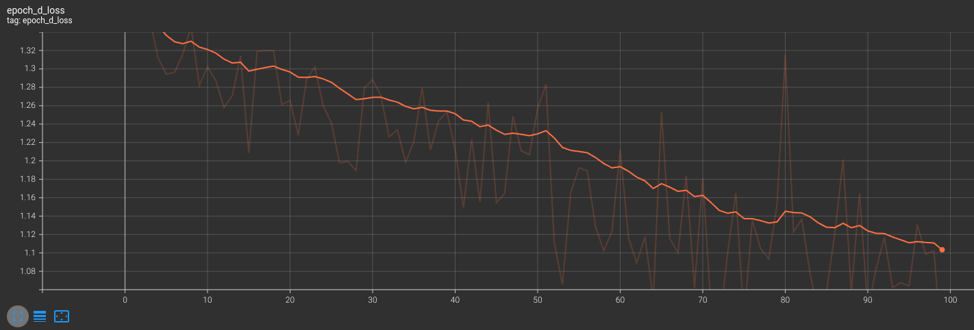
When training a DCGAN (Deep Convolutional Generative Adversarial Network) for image generation, the discriminator loss should ideally decrease over time as the discriminator gets better at distinguishing real images from fake ones generated by the generator. That's exactly what we can see in the image above.

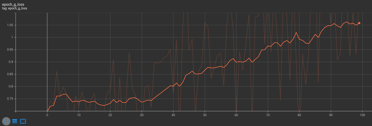
In general, we expect both the discriminator and generator losses to decrease over time as the DCGAN becomes better at generating realistic images. However, the specific values of the losses will depend on the architecture of our DCGAN and the quality of your training data. As we can see, our discriminator loss keeps decreasing while the generator keeps increasing over time. We would need to adjust our models. Still, because our dataset is relatively simple, we are not doing so... Increasing generator loss may indicate that our images need to be more realistic but let's see our results before making any decision.

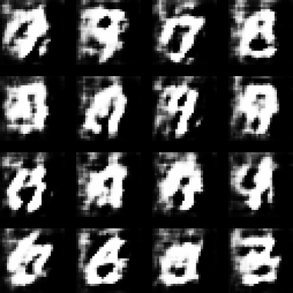
Here is generated GIF image from all the training epochs (100):

Conclusion:

In conclusion, this tutorial has introduced you to Generative Adversarial Networks in TensorFlow using the MNIST dataset. By following the step-by-step process, you've learned how to define the generator and discriminator models, create custom TensorFlow models, and use callbacks to track the training process.

You now have a basic understanding of how GANs work and how they can be used to generate new data similar to the training data. With this knowledge, you can further explore and experiment with GANs to generate more complex and diverse data in the future.

In the next tutorial, we'll cover some techniques and improvements to our GAN model so we could use it with way more challenging datasets, such as CelebA - to generate fake people portrait images.

The complete code for this tutorial you can find in this GitHub link.