Neural Network Backward propagation and parameters update

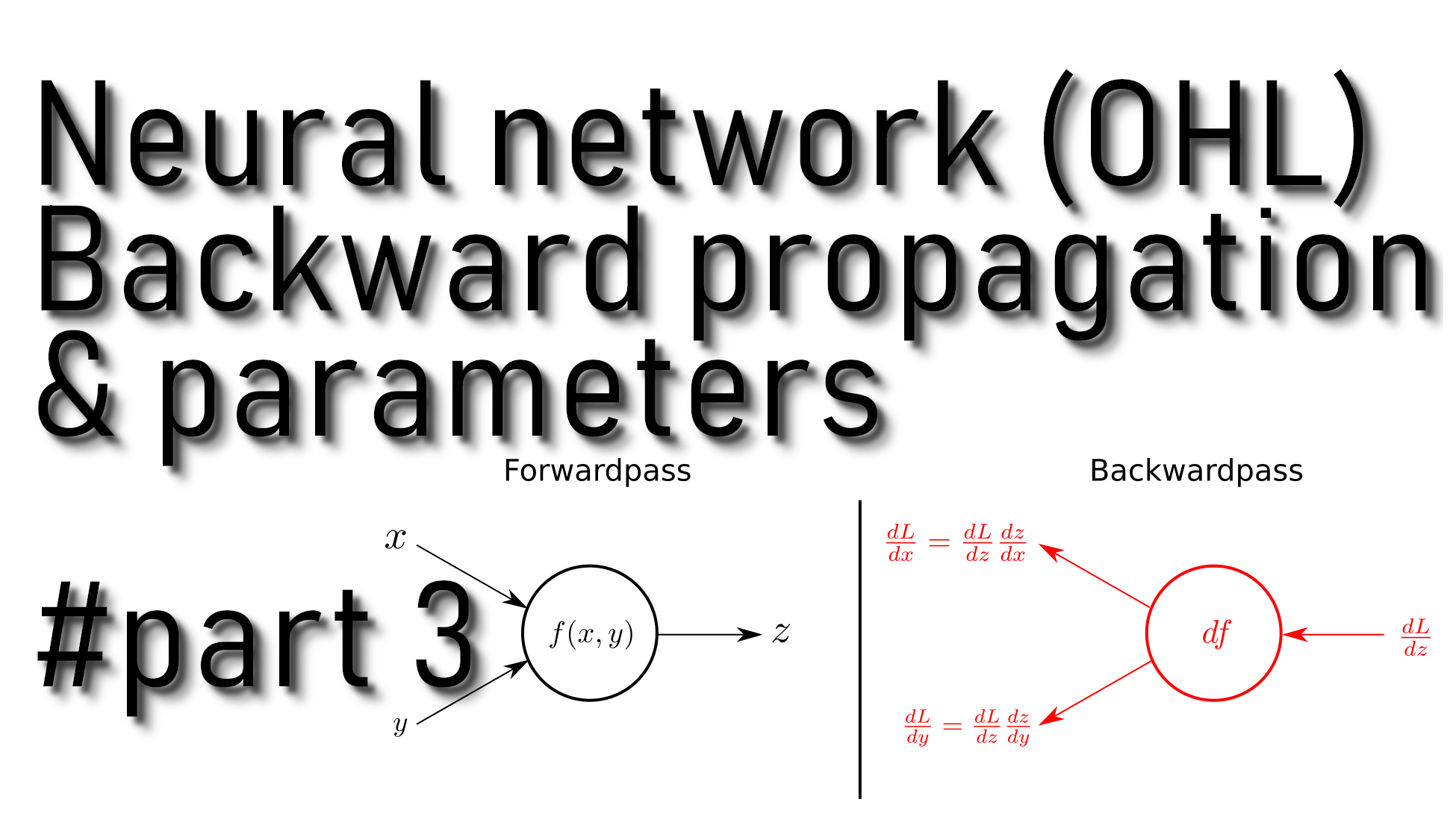
In our previous tutorial, we wrote forward propagation and cost functions. So next, we need to write a backpropagation function. For this, we'll use cache computed during the forward propagation.

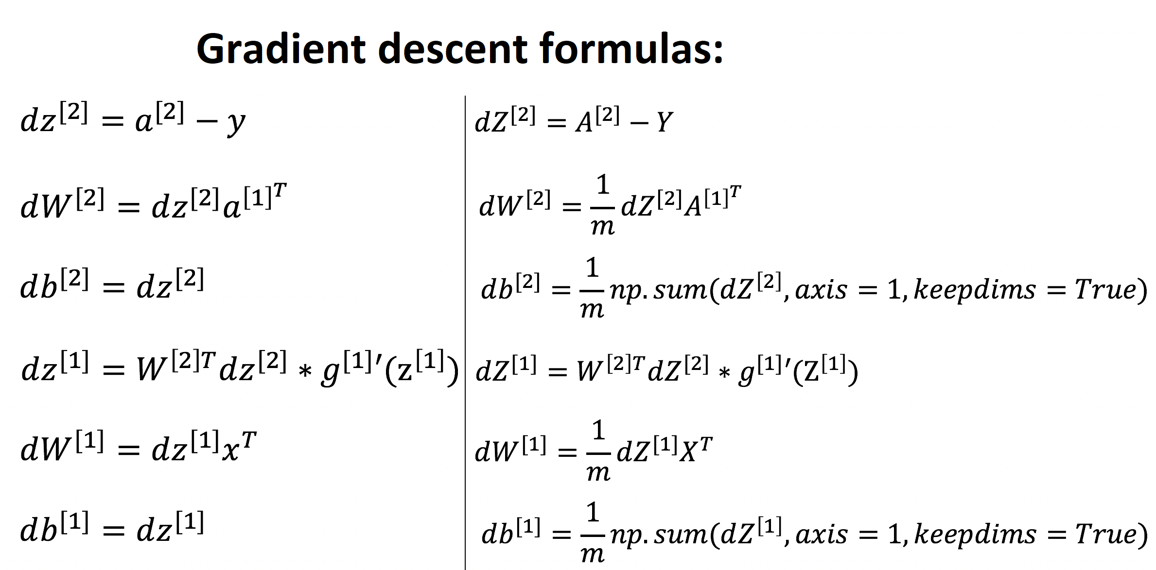
Backpropagation is usually the hardest (most mathematical) part of deep learning. Here again, is the picture with six mathematical equations we'll use. We'll use six equations on the right of this image since we are building a vectorized implementation.

Code for our backward propagation function:

Arguments:

parameters - python dictionary containing our parameters;
cache - a dictionary containing "Z1", "A1", "Z2" and "A2";
X - input data of shape (input, number of examples);
Y - "true" labels vector of shape (1, number of examples).

Return:

grads - python dictionary containing our gradients with respect to different parameters.

def backward_propagation(parameters, cache, X, Y):
    # number of example
    m = X.shape[1]
    
    # Retrieve W1 and W2 from the "parameters" dictionary
    W1 = parameters["W1"]
    W2 = parameters["W2"]

    # Retrieve A1 and A2 from "cache" dictionary
    A1 = cache["A1"]
    A2 = cache["A2"]

    # Backward propagation for dW1, db1, dW2, db2
    dZ2 = A2-Y
    dW2 = 1./m*np.dot(dZ2, A1.T)
    db2 = 1./m*np.sum(dZ2, axis = 1, keepdims=True)
    dZ1 = np.dot(W2.T, dZ2) * (1 - np.power(A1, 2))
    dW1 = 1./m*np.dot(dZ1, X.T)
    db1 = 1./m*np.sum(dZ1, axis = 1, keepdims=True)
    
    grads = {"dW1": dW1,
             "db1": db1,
             "dW2": dW2,
             "db2": db2}
    
    return grads

Code for our update parameters function:

We'll implement the update rule using gradient descent. So we'll have to use (dW1, db1, dW2, db2) to update (W1, b1, W2, b2).

$$\begin{gathered} \text{General Gradient descent rule is:} \\ \theta =\theta -\alpha \frac{\partial J}{\partial \theta } \\ \text{where}: \alpha - \text{learning rate}, \theta \text{represents a parameter} \end{gathered}$$

Arguments:

parameters - python dictionary containing our parameters;
grads - python dictionary containing your gradients;
learning_rate - learning rate of the gradient descent update rule;

Return:

parameters -- python dictionary containing your updated parameters

def update_parameters(parameters, grads, learning_rate = 0.1):
    # Retrieve each parameter from the dictionary "parameters"
    W1 = parameters["W1"]
    W2 = parameters["W2"]
    b1 = parameters["b1"]
    b2 = parameters["b2"]

    # Retrieve each gradient from the "grads" dictionary
    dW1 = grads["dW1"]
    db1 = grads["db1"]
    dW2 = grads["dW2"]
    db2 = grads["db2"]

    # Update rule for each parameter
    W1 = W1 - dW1 * learning_rate
    b1 = b1 - db1 * learning_rate
    W2 = W2 - dW2 * learning_rate
    b2 = b2 - db2 * learning_rate
    
    parameters = {"W1": W1,
                  "b1": b1,
                  "W2": W2,
                  "b2": b2}
    
    return parameters

Full tutorial code:

import os
import cv2
import numpy as np
import matplotlib.pyplot as plt
import scipy

ROWS = 64
COLS = 64
CHANNELS = 3

#TRAIN_DIR = 'Train_data/'
#TEST_DIR = 'Test_data/'

#train_images = [TRAIN_DIR+i for i in os.listdir(TRAIN_DIR)]
#test_images =  [TEST_DIR+i for i in os.listdir(TEST_DIR)]

def read_image(file_path):
    img = cv2.imread(file_path, cv2.IMREAD_COLOR)
    return cv2.resize(img, (ROWS, COLS), interpolation=cv2.INTER_CUBIC)

def prepare_data(images):
    m = len(images)
    X = np.zeros((m, ROWS, COLS, CHANNELS), dtype=np.uint8)
    y = np.zeros((1, m))
    for i, image_file in enumerate(images):
        X[i,:] = read_image(image_file)
        if 'dog' in image_file.lower():
            y[0, i] = 1
        elif 'cat' in image_file.lower():
            y[0, i] = 0
    return X, y

def sigmoid(z):
    s = 1/(1+np.exp(-z))
    return s
'''
train_set_x, train_set_y = prepare_data(train_images)
test_set_x, test_set_y = prepare_data(test_images)

train_set_x_flatten = train_set_x.reshape(train_set_x.shape[0], ROWS*COLS*CHANNELS).T
test_set_x_flatten = test_set_x.reshape(test_set_x.shape[0], -1).T

train_set_x = train_set_x_flatten/255
test_set_x = test_set_x_flatten/255
'''
#train_set_x_flatten shape: (12288, 6002)
#train_set_y shape: (1, 6002)

def initialize_parameters(input_layer, hidden_layer, output_layer):
    # initialize 1st layer output and input with random values
    W1 = np.random.randn(hidden_layer, input_layer) * 0.01
    # initialize 1st layer output bias
    b1 = np.zeros((hidden_layer, 1))
    # initialize 2nd layer output and input with random values
    W2 = np.random.randn(output_layer, hidden_layer) * 0.01
    # initialize 2nd layer output bias
    b2 = np.zeros((output_layer,1))
    
    parameters = {"W1": W1,
                  "b1": b1,
                  "W2": W2,
                  "b2": b2}
    
    return parameters

def forward_propagation(X, parameters):
    # Retrieve each parameter from the dictionary "parameters"
    W1 = parameters["W1"]
    b1 = parameters["b1"]
    W2 = parameters["W2"]
    b2 = parameters["b2"]

    # Implementing Forward Propagation to calculate A2 probabilities
    Z1 = np.dot(W1, X) + b1
    A1 =  np.tanh(Z1)
    Z2 = np.dot(W2, A1) + b2
    A2 = sigmoid(Z2)

    # Values needed in the backpropagation are stored in "cache"
    cache = {"Z1": Z1,
             "A1": A1,
             "Z2": Z2,
             "A2": A2}
    
    return A2, cache

def compute_cost(A2, Y, parameters):
    # number of example
    m = Y.shape[1]

    # Compute the cross-entropy cost
    logprobs = np.multiply(np.log(A2),Y) +  np.multiply(np.log(1-A2), (1-Y))
    cost = -1/m*np.sum(logprobs)

    # makes sure cost is in dimension we expect, E.g., turns [[51]] into 51 
    cost = np.squeeze(cost)
    
    return cost

def backward_propagation(parameters, cache, X, Y):
    # number of example
    m = X.shape[1]
    
    # Retrieve W1 and W2 from the "parameters" dictionary
    W1 = parameters["W1"]
    W2 = parameters["W2"]

    # Retrieve A1 and A2 from "cache" dictionary
    A1 = cache["A1"]
    A2 = cache["A2"]

    # Backward propagation for dW1, db1, dW2, db2
    dZ2 = A2-Y
    dW2 = 1./m*np.dot(dZ2, A1.T)
    db2 = 1./m*np.sum(dZ2, axis = 1, keepdims=True)
    dZ1 = np.dot(W2.T, dZ2) * (1 - np.power(A1, 2))
    dW1 = 1./m*np.dot(dZ1, X.T)
    db1 = 1./m*np.sum(dZ1, axis = 1, keepdims=True)
    
    grads = {"dW1": dW1,
             "db1": db1,
             "dW2": dW2,
             "db2": db2}
    
    return grads

def update_parameters(parameters, grads, learning_rate = 0.1):
    # Retrieve each parameter from "parameters" dictionary
    W1 = parameters["W1"]
    W2 = parameters["W2"]
    b1 = parameters["b1"]
    b2 = parameters["b2"]

    # Retrieve each gradient from the "grads" dictionary
    dW1 = grads["dW1"]
    db1 = grads["db1"]
    dW2 = grads["dW2"]
    db2 = grads["db2"]

    # Update rule for each parameter
    W1 = W1 - dW1 * learning_rate
    b1 = b1 - db1 * learning_rate
    W2 = W2 - dW2 * learning_rate
    b2 = b2 - db2 * learning_rate
    
    parameters = {"W1": W1,
                  "b1": b1,
                  "W2": W2,
                  "b2": b2}
    
    return parameters