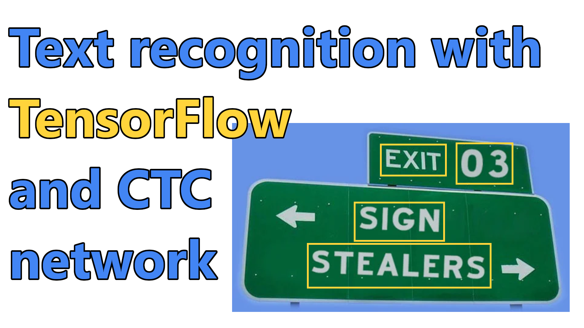
If you came to this article, you should know that extracting text from images is a complex problem. Extracting text of different sizes, shapes, and orientations from images is a fundamental problem in many contexts, especially in augmented reality assistance systems, e-commerce, and content moderation on social media platforms. To solve this problem, we need to extract text from images accurately.
There are two most popular methods that we could use to extract text from images:
- We can localize text in images using text detectors or segmentation techniques, then extract localized text (more straightforward way);
- We can train a model that achieves both text detection and recognition within a single model (the hard way);
In this tutorial, I will focus only on a word extraction part from the whole OCR pipeline:
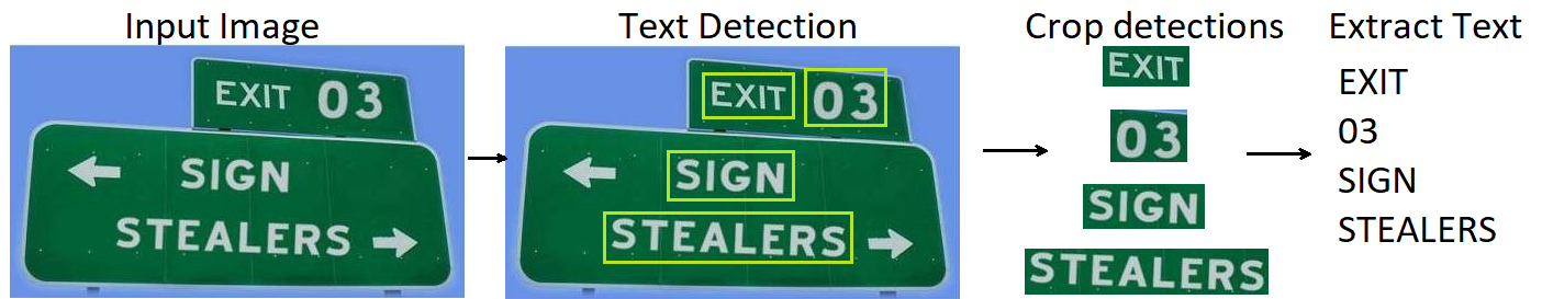
But, it's valuable to know the pipeline of the most popular OCRs available today. As I said, most pipelines contain a Text Detection step and Text Recognition steps:
- Text Detection helps you identify the location of an image that contains the text. It takes an image as input and gives boxes with coordinates as output;
- Text Recognition extracts text from an input image using bounding boxes derived from a text detection model. It inputs an image with cropped image parts using the bounding boxes from the detector and outputs raw text.
Text detection is very similar to the Object Detection task, where the object which needs to be detected is nothing but the text. Much research has taken place in this field to detect text out of images accurately, and many detectors detect text at the word level. However, the problem with word-level detectors is that they fail to notice words of arbitrary shape (rotated, curved, stretched, etc.).
But it was proven that we could achieve even better results by using various segmentation techniques instead of using detectors. Exploring each character and the spacings between characters helps to detect various shaped texts.[1]
For text detection, you can choose other popular techniques. But, as I already mentioned, it would be too complex and an extensive tutorial to cover both. So, I will focus on explaining the CTC networks for text recognition.
I noticed that when developing various things, I must reimplement things I was already using over and over. So why not simplify this by creating a library to hold all this stuff? With this tutorial, I am starting a new MLTU (Machine Learning Training Utilities) library that I will open source on GitHub, where I'll save all tutorial code there.
Text Recognition Pipeline:
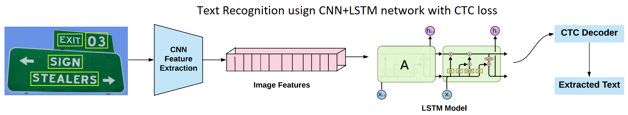
After the text localization step, regions containing text are cropped and sent through CNN layers to extract image features. These features are later fed into a many-to-many LSTM architecture that outputs softmax probabilities via a dictionary. These outputs at different time steps are provided to the CTC decoder to obtain the raw text from the images. I will cover each step in detail in the following sections of the tutorial.
First, let us look at my TensorFlow model to understand how we connect the CNN layers with LSTM layers. This tutorial is not beginner-level, so I'll only cover some parts step by step, and I'll only post some of the code here, deeper code parts, you can look at my GitHub repository.
Files for this tutorial you can find on https://github.com/pythonlessons/mltu/tree/main/Tutorials/01_image_to_word link. To run this tutorial, you must install my "mltu" 0.1.3 version package with pip:
pip install mltu==0.1.3
Here is the code to construct our model in TensorFlow:
# Tutorials/01_image_to_word/model.py
from keras import layers
from keras.models import Model

from mltu.model_utils import residual_block

def train_model(input_dim, output_dim, activation='leaky_relu', dropout=0.2):

    inputs = layers.Input(shape=input_dim, name="input")

    input = layers.Lambda(lambda x: x / 255)(inputs)

    x1 = residual_block(input, 16, activation=activation, skip_conv=True, strides=1, dropout=dropout)

    x2 = residual_block(x1, 16, activation=activation, skip_conv=True, strides=2, dropout=dropout)
    x3 = residual_block(x2, 16, activation=activation, skip_conv=False, strides=1, dropout=dropout)

    x4 = residual_block(x3, 32, activation=activation, skip_conv=True, strides=2, dropout=dropout)
    x5 = residual_block(x4, 32, activation=activation, skip_conv=False, strides=1, dropout=dropout)

    x6 = residual_block(x5, 64, activation=activation, skip_conv=True, strides=1, dropout=dropout)
    x7 = residual_block(x6, 64, activation=activation, skip_conv=False, strides=1, dropout=dropout)

    squeezed = layers.Reshape((x7.shape[-3] * x7.shape[-2], x7.shape[-1]))(x7)

    blstm = layers.Bidirectional(layers.LSTM(64, return_sequences=True))(squeezed)

    output = layers.Dense(output_dim + 1, activation='softmax', name="output")(blstm)

    model = Model(inputs=inputs, outputs=output)
    return model
I used a principle from ResNet models to construct residual blocks that help our model to learn better details. I'll resize all the input images to 32 by 128 pixels. With this size, our model summary will look following:
 Layer (type)                                    Output Shape                     Param #           Connected to
======================================================================================================================================================
 input (InputLayer)                              [(None, 32, 128, 3)]             0                 []
 lambda (Lambda)                                 (None, 32, 128, 3)               0                 ['input[0][0]']
 conv2d (Conv2D)                                 (None, 32, 128, 16)              448               ['lambda[0][0]']
 batch_normalization (BatchNormalization)        (None, 32, 128, 16)              64                ['conv2d[0][0]']
 leaky_re_lu (LeakyReLU)                         (None, 32, 128, 16)              0                 ['batch_normalization[0][0]']
 conv2d_1 (Conv2D)                               (None, 32, 128, 16)              2320              ['leaky_re_lu[0][0]']
 batch_normalization_1 (BatchNormalization)      (None, 32, 128, 16)              64                ['conv2d_1[0][0]']
 conv2d_2 (Conv2D)                               (None, 32, 128, 16)              64                ['lambda[0][0]']
 add (Add)                                       (None, 32, 128, 16)              0                 ['batch_normalization_1[0][0]',
                                                                                                     'conv2d_2[0][0]']
 leaky_re_lu_1 (LeakyReLU)                       (None, 32, 128, 16)              0                 ['add[0][0]']
 dropout (Dropout)                               (None, 32, 128, 16)              0                 ['leaky_re_lu_1[0][0]']
 conv2d_3 (Conv2D)                               (None, 16, 64, 16)               2320              ['dropout[0][0]']
 batch_normalization_2 (BatchNormalization)      (None, 16, 64, 16)               64                ['conv2d_3[0][0]']
 leaky_re_lu_2 (LeakyReLU)                       (None, 16, 64, 16)               0                 ['batch_normalization_2[0][0]']
 conv2d_4 (Conv2D)                               (None, 16, 64, 16)               2320              ['leaky_re_lu_2[0][0]']
 batch_normalization_3 (BatchNormalization)      (None, 16, 64, 16)               64                ['conv2d_4[0][0]']
 conv2d_5 (Conv2D)                               (None, 16, 64, 16)               272               ['dropout[0][0]']
 add_1 (Add)                                     (None, 16, 64, 16)               0                 ['batch_normalization_3[0][0]',
                                                                                                     'conv2d_5[0][0]']
 leaky_re_lu_3 (LeakyReLU)                       (None, 16, 64, 16)               0                 ['add_1[0][0]']
 dropout_1 (Dropout)                             (None, 16, 64, 16)               0                 ['leaky_re_lu_3[0][0]']
 conv2d_6 (Conv2D)                               (None, 16, 64, 16)               2320              ['dropout_1[0][0]']
 batch_normalization_4 (BatchNormalization)      (None, 16, 64, 16)               64                ['conv2d_6[0][0]']
 leaky_re_lu_4 (LeakyReLU)                       (None, 16, 64, 16)               0                 ['batch_normalization_4[0][0]']
 conv2d_7 (Conv2D)                               (None, 16, 64, 16)               2320              ['leaky_re_lu_4[0][0]']
 batch_normalization_5 (BatchNormalization)      (None, 16, 64, 16)               64                ['conv2d_7[0][0]']
 add_2 (Add)                                     (None, 16, 64, 16)               0                 ['batch_normalization_5[0][0]',
                                                                                                     'dropout_1[0][0]']
 leaky_re_lu_5 (LeakyReLU)                       (None, 16, 64, 16)               0                 ['add_2[0][0]']
 dropout_2 (Dropout)                             (None, 16, 64, 16)               0                 ['leaky_re_lu_5[0][0]']
 conv2d_8 (Conv2D)                               (None, 8, 32, 32)                4640              ['dropout_2[0][0]']
 batch_normalization_6 (BatchNormalization)      (None, 8, 32, 32)                128               ['conv2d_8[0][0]']
 leaky_re_lu_6 (LeakyReLU)                       (None, 8, 32, 32)                0                 ['batch_normalization_6[0][0]']
 conv2d_9 (Conv2D)                               (None, 8, 32, 32)                9248              ['leaky_re_lu_6[0][0]']
 batch_normalization_7 (BatchNormalization)      (None, 8, 32, 32)                128               ['conv2d_9[0][0]']
 conv2d_10 (Conv2D)                              (None, 8, 32, 32)                544               ['dropout_2[0][0]']
 add_3 (Add)                                     (None, 8, 32, 32)                0                 ['batch_normalization_7[0][0]',
                                                                                                     'conv2d_10[0][0]']
 leaky_re_lu_7 (LeakyReLU)                       (None, 8, 32, 32)                0                 ['add_3[0][0]']
 dropout_3 (Dropout)                             (None, 8, 32, 32)                0                 ['leaky_re_lu_7[0][0]']
 conv2d_11 (Conv2D)                              (None, 8, 32, 32)                9248              ['dropout_3[0][0]']
 batch_normalization_8 (BatchNormalization)      (None, 8, 32, 32)                128               ['conv2d_11[0][0]']
 leaky_re_lu_8 (LeakyReLU)                       (None, 8, 32, 32)                0                 ['batch_normalization_8[0][0]']
 conv2d_12 (Conv2D)                              (None, 8, 32, 32)                9248              ['leaky_re_lu_8[0][0]']
 batch_normalization_9 (BatchNormalization)      (None, 8, 32, 32)                128               ['conv2d_12[0][0]']
 add_4 (Add)                                     (None, 8, 32, 32)                0                 ['batch_normalization_9[0][0]',
                                                                                                     'dropout_3[0][0]']
 leaky_re_lu_9 (LeakyReLU)                       (None, 8, 32, 32)                0                 ['add_4[0][0]']
 dropout_4 (Dropout)                             (None, 8, 32, 32)                0                 ['leaky_re_lu_9[0][0]']
 conv2d_13 (Conv2D)                              (None, 8, 32, 64)                18496             ['dropout_4[0][0]']
 batch_normalization_10 (BatchNormalization)     (None, 8, 32, 64)                256               ['conv2d_13[0][0]']
 leaky_re_lu_10 (LeakyReLU)                      (None, 8, 32, 64)                0                 ['batch_normalization_10[0][0]']
 conv2d_14 (Conv2D)                              (None, 8, 32, 64)                36928             ['leaky_re_lu_10[0][0]']
 batch_normalization_11 (BatchNormalization)     (None, 8, 32, 64)                256               ['conv2d_14[0][0]']
 conv2d_15 (Conv2D)                              (None, 8, 32, 64)                2112              ['dropout_4[0][0]']
 add_5 (Add)                                     (None, 8, 32, 64)                0                 ['batch_normalization_11[0][0]',
                                                                                                     'conv2d_15[0][0]']
 leaky_re_lu_11 (LeakyReLU)                      (None, 8, 32, 64)                0                 ['add_5[0][0]']
 dropout_5 (Dropout)                             (None, 8, 32, 64)                0                 ['leaky_re_lu_11[0][0]']
 conv2d_16 (Conv2D)                              (None, 8, 32, 64)                36928             ['dropout_5[0][0]']
 batch_normalization_12 (BatchNormalization)     (None, 8, 32, 64)                256               ['conv2d_16[0][0]']
 leaky_re_lu_12 (LeakyReLU)                      (None, 8, 32, 64)                0                 ['batch_normalization_12[0][0]']
 conv2d_17 (Conv2D)                              (None, 8, 32, 64)                36928             ['leaky_re_lu_12[0][0]']
 batch_normalization_13 (BatchNormalization)     (None, 8, 32, 64)                256               ['conv2d_17[0][0]']
 add_6 (Add)                                     (None, 8, 32, 64)                0                 ['batch_normalization_13[0][0]',
                                                                                                     'dropout_5[0][0]']
 leaky_re_lu_13 (LeakyReLU)                      (None, 8, 32, 64)                0                 ['add_6[0][0]']
 dropout_6 (Dropout)                             (None, 8, 32, 64)                0                 ['leaky_re_lu_13[0][0]']
 reshape (Reshape)                               (None, 256, 64)                  0                 ['dropout_6[0][0]']
 bidirectional (Bidirectional)                   (None, 256, 128)                 66048             ['reshape[0][0]']
 output (Dense)                                  (None, 256, 63)                  8127              ['bidirectional[0][0]']
======================================================================================================================================================
Total params: 252,799
Trainable params: 251,839
Non-trainable params: 960
______________________________________________________________________________________________________________________________________________________
This may give you limited information if you are unfamiliar with TensorFlow, but the idea here is to create a model with the correct output for our CTC loss function. To do so, we must transition from CNN to LSTM layers. To do so, I used a reshaped CNN last layer to remove one dimension, which would be great for LSTM input.
To make everything right, we must ensure that the last layer meets the requirements of the CTC loss function. Here I have 63; in my words dataset, I know I have 62 different characters, but we need to increment it by 1 (separation token). I also have 256; as you may see here, we must ensure that this value is greater than the maximum word length in our dataset, which in mine is 23. This one will be seen as spacing in our prediction; more about it later.
First, let's understand the concept of receptive fields to make it easier to understand how the features of a CNN model are transferred to an LSTM network.
CNN Features to LSTM layer:
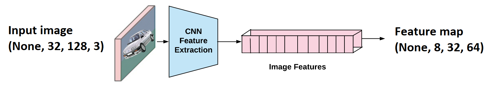
The above image shows that an image (32x128 size) is sent through convolutional layers. Layers are designed so that, as a result, we obtain feature maps of the shape (None, 8, 32, 64). "None" here is the batch size that could take any value.
(None, 8, 32, 64) can be easily reshaped to (None, 256, 64), and 256 corresponds to the number of time steps, and 64 is nothing but the number of features at every time step. One can relate this to training any LSTM model with word embeddings, and the input shape is usually (batch_size, no_time_steps, word_embedding_dimension).
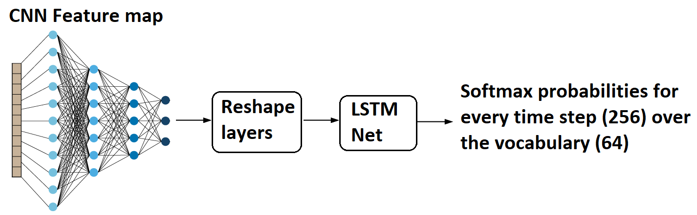
Later these feature maps are fed to the LSTM model, as shown above. You might be thinking now that LSTM models are known to work with sequential data and how feature maps are sequential. But the idea here is that CNN layers reshape the sequences while changing the view with its layers.
As a result, we get a softmax probability over vocabulary from the LSTM model for every time step, i.e., 256. Now let us move on to the exciting part of the tutorial on calculating the loss value for this architecture setup.
What is CTC loss, and why do we use it:
This is an extensive topic for which I could create another whole explanation tutorial. But because there is already plenty of articles about CTC loss, I'll mention only the entire idea.
Of course, we could create a dataset with images of text strings and then specify the corresponding symbol for each horizontal image position. We could train the NN to output the character score for each horizontal position using the categorical cross-entropy as the loss. However, there are a few problems with this solution:
- It is very time-consuming (and tedious) to annotate a data set at the character level;
- We only get character scores and need further processing to get the final text. We need to remove all duplicate characters. A single symbol can take multiple horizontal positions; For example, we can get "Heeloo" because "e" or "e" is wide. But what if the recognized text had been "Good"? Then removing all the repeated 'o's gives us an incorrect result. How to handle it?
- Mentioned CTC loss is suitable for speech-to-text applications as well. Audio signal and corresponding text are available as training data, and there is no mapping like the first character is spoken for "x" milliseconds or from "x1" to "x2" milliseconds character "z" is spoken. It would be impossible to annotate each character's sound words in time series.
CTC solves all of these problems for us:
- While training the model with the CTC loss function, we only need to know the exact word in the image. Therefore, we ignore both the position and the width of the symbols in the image or audio spectrogram;
- The recognized text does not require further processing.
To distinguish between two consecutive tokens and duplicate tokens, a "separation" token is used, as I already mentioned before. The best way to understand how it works would be to imagine that we are working with sound data that says the word "Good":
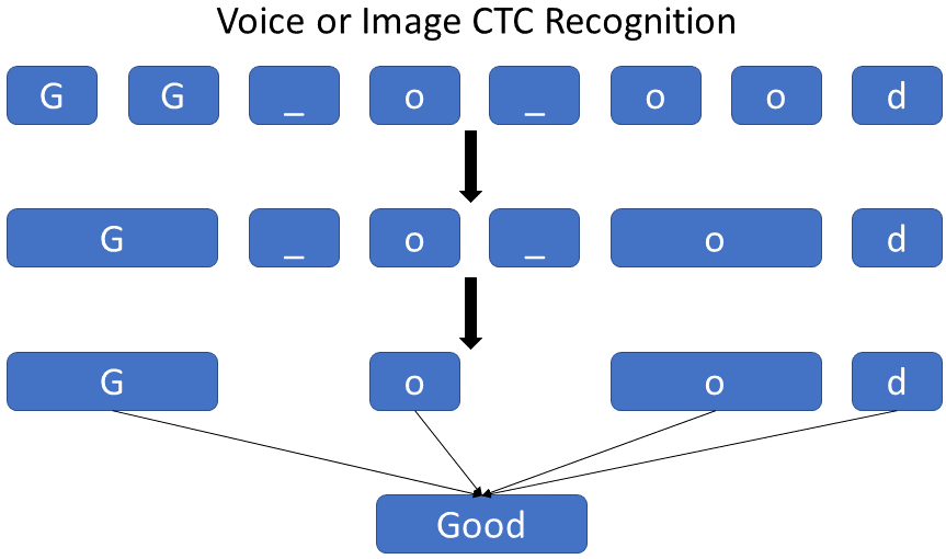
We use a clever encoding scheme to solve the problem of duplicate characters. When encoding a text, we can insert an arbitrary number of blanks at any place, which will be removed when decoding it. Also, we can repeat each character as many times as we want. However, we need to insert a blank space between repeated symbols, like "Hello".
We can create a few examples:
- From word Home → "H-o-m-e", "H-ooo-m-ee", "-HHHHHHo-m-e", etc.;
- from word Good → "G-o-o-d", "GGGo-od", "G-ooooo-oooo-dddd", etc.;
As you see, this technique also allows us to create different alignments of the exact text easily, e.g., "H-o-m-e", "H-ooo-m-ee", "-HHHHHHo-m-e" all represent the actual text (Home), but with different alignments to the image. The Neural Network has been trained to output the scrambled text (encoded in the NN softmax output).
Once we have a trained Neural Network, we typically want to use it to recognize text in images that our model has never seen. A simple and very fast algorithm is the "best path decoding", consisting of two steps:
- It calculates the best path based on the most probable symbol per time step;
- It undoes the encoding by removing duplicate characters and all blanks from the path. What remains represents the recognized text!
That's a short cover about CTC loss not getting into the math, but if you are interested to understand and study how math works, I found this great article that explains it step by step.
CTC loss code:
Let's get back to the coding part. I'll only be coding some of the math calculations covered before. We can use the "keras.backend.ctc_batch_cost" function for calculating the CTC loss, and below is the code for the same where a custom CTC layer is defined, which is used in both training and evaluation parts. To use it as a loss function, we need to construct an inheritance object to do so:
import tensorflow as tf

class CTCloss(tf.keras.losses.Loss):
    """ CTCLoss objec for training the model"""
    def __init__(self, name: str = 'CTCloss') -> None:
        super(CTCloss, self).__init__()
        self.name = name
        self.loss_fn = tf.keras.backend.ctc_batch_cost

    def __call__(self, y_true: tf.Tensor, y_pred: tf.Tensor, sample_weight=None) -> tf.Tensor:
        """ Compute the training batch CTC loss value"""
        batch_len = tf.cast(tf.shape(y_true)[0], dtype="int64")
        input_length = tf.cast(tf.shape(y_pred)[1], dtype="int64")
        label_length = tf.cast(tf.shape(y_true)[1], dtype="int64")

        input_length = input_length * tf.ones(shape=(batch_len, 1), dtype="int64")
        label_length = label_length * tf.ones(shape=(batch_len, 1), dtype="int64")

        loss = self.loss_fn(y_true, y_pred, input_length, label_length)

        return loss
Now, when we are constructing and compiling our model, we use it as a regular loss function:
# Tutorials/01_image_to_word/train.py
model = train_model(
    input_dim = (configs.height, configs.width, 3),
    output_dim = len(configs.vocab),
)
# Compile the model and print summary
model.compile(
    optimizer=tf.keras.optimizers.Adam(learning_rate=configs.learning_rate),
    loss=CTCloss(),
    metrics=[CWERMetric()],
)
That's it; our model is ready to be fed with images and annotations and to be trained. But you may notice that I use some CWER metric. That's right! While training word, speech, and sentence recognition models, it's not a good practice to rely simply on a validation loss. Knowing how many mistakes our model makes in the validation dataset is better. This way, we'll be able to enhance our model architecture for better results.
Not to waste our resources, I implemented it as a TensorFlow metric to run as it trains.
Character Error Rate (CER) measures the accuracy of a transcription or translation, typically used in speech recognition or natural language processing. It compares the ground truth transcription or translation (the correct version) to the actual transcription or translation produced by a system and calculates the percentage of errors in the output.
To calculate CER, we first count the total number of characters in the ground truth transcription or translation, including spaces. We then count the number of insertions, substitutions, and deletions of characters that are required to transform the output transcription or translation into the ground truth. The CER is then calculated as the sum of these errors divided by the total number of characters, expressed as a percentage.
In other words, CER measures the number of errors in the output transcription or translation relative to the total number of characters in the ground truth. It considers mistakes in spelling or grammar but also missing or extra spaces, capitalization errors, and other minor transcription mismatches.
For example, suppose we have the following ground truth transcription: "This is a test sentence."
And suppose we have the following output transcription produced by a speech recognition system: "This is a test sentence."
In this case, the output transcription is the same as the ground truth, so there are no errors. The CER would be 0%.
On the other hand, if we had the following output transcription: "This is a test sentenee."
There is a single character error (an extra "e" at the end of the sentence), so the CER would be 1/23 = 4.3%.
Training callbacks:
You may have noticed that I utilize several callbacks in my code on GitHub. Callbacks are groups of functions that are implemented at specific stages of the training process. These callbacks allow you to observe the statistics and internal states of the model during training.
I tend to use callbacks in almost all of my trainable models."
# Define callbacks
earlystopper = EarlyStopping(monitor='val_CER', patience=10, verbose=1)
checkpoint = ModelCheckpoint(f"{configs.model_path}/model.h5", monitor='val_CER', verbose=1, save_best_only=True, mode='min')
trainLogger = TrainLogger(configs.model_path)
tb_callback = TensorBoard(f'{configs.model_path}/logs', update_freq=1)
reduceLROnPlat = ReduceLROnPlateau(monitor='val_CER', factor=0.9, min_delta=1e-10, patience=5, verbose=1, mode='auto')
model2onnx = Model2onnx(f"{configs.model_path}/model.h5")
We can count six different callbacks that speak for themselves, and as you may see, instead of tracking validation loss, I am following validation CER ("val_CER")!
Most of us train these models to deploy somewhere we don't want to use TensorFlow installed. So, I created a "Model2onxx" callback that, at the end of the training, converts the model to .onnx format, which can be used without this huge TensorFlow library, and usually, it runs twice faster!
Preparing the dataset:
This is another broad topic that I'll try to cover quickly by mentioning only the most essential aspects. So, for this tutorial, we are creating a model to recognize text from simple text images. I found a vast "Text Recognition data" database that lets us do so.
This dataset consists of 9 million images covering 90k English words and includes the training, validation, and test splits used in our work.
If you are following my tutorial, download this 10 GB dataset and extract it to the "Datasets/90kDICT32px" folder.
With the following code, we'll read all the paths for our training and validation dataset:
# Tutorials/01_image_to_word/train.py
configs = ModelConfigs()

data_path = "Datasets/90kDICT32px"
val_annotation_path = data_path + "/annotation_val.txt"
train_annotation_path = data_path + "/annotation_train.txt"

# Read metadata file and parse it
def read_annotation_file(annotation_path):
    dataset, vocab, max_len = [], set(), 0
    with open(annotation_path, "r") as f:
        for line in tqdm(f.readlines()):
            line = line.split()
            image_path = data_path + line[0][1:]
            label = line[0].split("_")[1]
            dataset.append([image_path, label])
            vocab.update(list(label))
            max_len = max(max_len, len(label))
    return dataset, sorted(vocab), max_len

train_dataset, train_vocab, max_train_len = read_annotation_file(train_annotation_path)
val_dataset, val_vocab, max_val_len = read_annotation_file(val_annotation_path)

# Save vocab and maximum text length to configs
configs.vocab = "".join(train_vocab)
configs.max_text_length = max(max_train_len, max_val_len)
configs.save()
This is a simple for loop that, on each loop, reads the file path and extracts the actual label of the word. Also, we are collecting vocabulary and the maximum word length possible. The two parameters are later used to construct a proper model for our task.
Okay, next, we'll construct our training and validation data providers using the basic DataProvider model from my "mltu" package:
# Tutorials/01_image_to_word/train.py

# Create training data provider
train_data_provider = DataProvider(
    dataset=train_dataset,
    skip_validation=True,
    batch_size=configs.batch_size,
    data_preprocessors=[ImageReader()],
    transformers=[
        ImageResizer(configs.width, configs.height),
        LabelIndexer(configs.vocab),
        LabelPadding(max_word_length=configs.max_text_length, padding_value=len(configs.vocab))
        ],
)

# Create validation data provider
val_data_provider = DataProvider(
    dataset=val_dataset,
    skip_validation=True,
    batch_size=configs.batch_size,
    data_preprocessors=[ImageReader()],
    transformers=[
        ImageResizer(configs.width, configs.height),
        LabelIndexer(configs.vocab),
        LabelPadding(max_word_length=configs.max_text_length, padding_value=len(configs.vocab))
        ],
)
I created this object to make data providers for any data type using different data preprocessors, augmentors, or transformers.
Specifically for an image-to-text task, I am using a simple OpenCV "ImageReader" preprocessor. Then I use transformers to standardize our images and labels; first, we resize all images to the same size. Next, we convert string labels to indexes because our model doesn't understand string; it must be numeric values. And in the last step, we pad our words with unknown values so that our input meets the exact shape requirement.
Training the model:
We came to the point where we finally trained our model. Because it takes more than an hour to complete even a single epoch on my 1080TI GPU, I am not showing the whole training process. But because of our great callbacks, we can check our training logs and Tensorboard logs.
This is the code that we use to create mode, compile it, define callbacks and initiate the model training process:
# Tutorials/01_image_to_word/train.py
model = train_model(
    input_dim = (configs.height, configs.width, 3),
    output_dim = len(configs.vocab),
)
# Compile the model and print summary
model.compile(
    optimizer=tf.keras.optimizers.Adam(learning_rate=configs.learning_rate),
    loss=CTCloss(),
    metrics=[CWERMetric()],
    run_eagerly=False
)

# Define callbacks
earlystopper = EarlyStopping(monitor='val_CER', patience=10, verbose=1)
checkpoint = ModelCheckpoint(f"{configs.model_path}/model.h5", monitor='val_CER', verbose=1, save_best_only=True, mode='min')
trainLogger = TrainLogger(configs.model_path)
tb_callback = TensorBoard(f'{configs.model_path}/logs', update_freq=1)
reduceLROnPlat = ReduceLROnPlateau(monitor='val_CER', factor=0.9, min_delta=1e-10, patience=5, verbose=1, mode='auto')
model2onnx = Model2onnx(f"{configs.model_path}/model.h5")

# Train the model
model.fit(
    train_data_provider,
    validation_data=val_data_provider,
    epochs=configs.train_epochs,
    callbacks=[earlystopper, checkpoint, trainLogger, reduceLROnPlat, tb_callback, model2onnx],
    workers=configs.train_workers
)
Now, I can open the Tensorboard dashboard with the path of my trained model logs by issuing the following command in the terminal:
tensorboard --logdir Models/1_image_to_word/202211270035/logs
Because our dataset is huge, most of the things it learns in its first epoch, so when it finishes the first training epoch, our CER will give us pretty nice results:
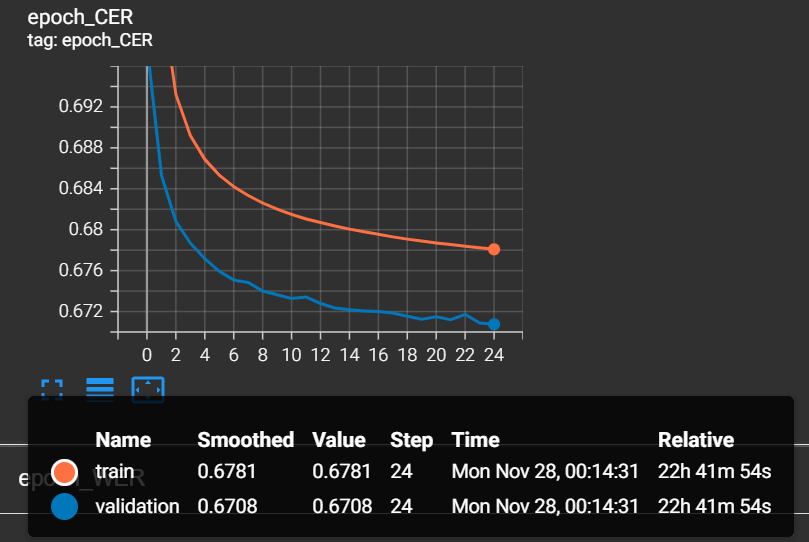
As we can see, in every epoch, our CER rate is decreasing. That's what we expect!
When our training process was finished, two models were saved: the default .h5 Keras model and the .onnx format model. So, let's run inference on our saved model.
Testing the model:
Nowadays, everyone knows how to run inference on the default ".h5" Keras model, but usually, it's not the best choice when we want to deploy our solutions somewhere. This is the reason why I convert the model to .onnx format. It's a lightweight model format that usually is faster and doesn't require huge libraries to install.
First, I am creating an object that will load the ".onnx" model and handle all the data preprocessing and post-processing. To do so, my object inherits from the "OnnxInferenceModel" object:
# Tutorials/01_image_to_word/inferenceModel.py
import cv2
import typing
import numpy as np

from mltu.inferenceModel import OnnxInferenceModel
from mltu.utils.text_utils import ctc_decoder, get_cer

class ImageToWordModel(OnnxInferenceModel):
    def __init__(self, char_list: typing.Union[str, list], *args, **kwargs):
        super().__init__(*args, **kwargs)
        self.char_list = char_list

    def predict(self, image: np.ndarray):
        image = cv2.resize(image, self.input_shape[:2][::-1])

        image_pred = np.expand_dims(image, axis=0).astype(np.float32)

        preds = self.model.run(None, {self.input_name: image_pred})[0]

        text = ctc_decoder(preds, self.char_list)[0]

        return text
The only thing we'll need to pass to ImageToWordModel while creating an object is vocabulary. That's why it's important to serialize and save configurations when training a model.
Now let's write a code to run inference on each image in our validation dataset and check what the Character Error Rate is:
# Tutorials/01_image_to_word/inferenceModel.py
if __name__ == "__main__":
    import pandas as pd
    from tqdm import tqdm
    from mltu.configs import BaseModelConfigs

    configs = BaseModelConfigs.load("Models/1_image_to_word/202211270035/configs.yaml")

    model = ImageToWordModel(model_path=configs.model_path, char_list=configs.vocab)

    df = pd.read_csv("Models/1_image_to_word/202211270035/val.csv").dropna().values.tolist()

    accum_cer = []
    for image_path, label in tqdm(df):
        image = cv2.imread(image_path)

        try:
            prediction_text = model.predict(image)

            cer = get_cer(prediction_text, label)
            print(f"Image: {image_path}, Label: {label}, Prediction: {prediction_text}, CER: {cer}")

            # resize image by 3 times for visualization
            # image = cv2.resize(image, (image.shape[1] * 3, image.shape[0] * 3))
            # cv2.imshow(prediction_text, image)
            # cv2.waitKey(0)
            # cv2.destroyAllWindows()
        except:
            continue

        accum_cer.append(cer)

    print(f"Average CER: {np.average(accum_cer)}")
I can run this for 1000 examples, and I'll receive the following results:
Average CER: 0.07760155677655678
This means that within 1000 examples, my model has 7% of CER; that's pretty good, knowing that our training and validation dataset could be better!
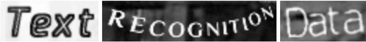
Here are a few examples:
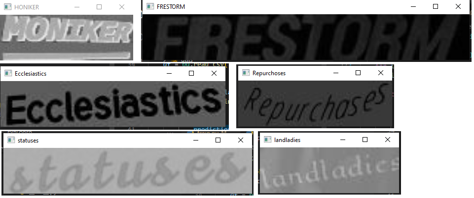 I showed here only a few examples. You can test this out with way more examples.
Conclusion:
In conclusion, extracting text from images is a complex problem that is important in various contexts, including augmented reality, e-commerce, and content moderation. There are two main approaches to extracting text from images: using text detectors or segmentation techniques to localize text and training a single model that performs text detection and recognition. This tutorial focuses on the latter approach, combining CNN and LSTM layers with a CTC loss function to extract text from images. The tutorial also introduces a new open-source library called MLTU (Machine Learning Training Utilities) that will be used to store code from future tutorials.
In this tutorial, I tried to be as short as possible and explain only the most essential parts. Going deeper, it could be expanded into several different tutorials, but I still need to do more. At the end of this tutorial, we finally have a working custom OCR model to recognize text from our Images.
This is the first part of my tutorial series, where we learned how to train our custom OCR to recognize text from our images. From now on, we can move to other, more challenging tasks.
I hope this tutorial was helpful for you, and you can use my code or even my new "mltu" (pip install mltu) package for your project. See you in the next tutorial!
The model I trained can be downloaded from this link (Place it in the Models folder). Have fun!