In the previous tutorial, I showed you how to make Handwritten word recognition. Now it's time for sentence recognition! That's a challenging task that involves interpreting text written in handwriting. This task has various applications, including converting handwritten notes into digital text, transcribing historical documents, automating the grading of exams, etc.

One of the critical challenges in handwritten sentence recognition is handwriting variability. People have different handwriting styles, and even the same person can have different handwriting styles at other times. This makes it difficult for a machine-learning model to recognize handwritten text accurately.

Researchers have developed various techniques and methods for handwritten sentence recognition to address this challenge. This tutorial will focus on one approach: TensorFlow and CTC loss for handwritten sentence recognition.

Challenges in Handwriting Sentence Recognition:

Try reading the following image:

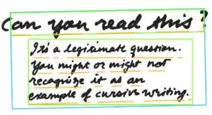It took you a few seconds, right? Properly trained machine learning could read this image and type what's written in milliseconds! But, we must address several challenges in handwritten sentence recognition to perform well. Some of these challenges include:

• The variability and ambiguity of strokes from person to person can make it difficult for a model to recognize the text accurately;
• The inconsistency of an individual's handwriting style, which can change over time and make it difficult for a model to recognize the text;
• Noise and deformations, such as smudges, creases, or ink blots, can impact the recognition process and make it difficult for a model to identify the text;
• The layout and context of the text, such as font or placement within a larger text block, can also impact the recognition process.
• Cursive handwriting makes separation and recognition of characters challenging;
• Handwritten text can appear at different angles, unlike printed text which is typically upright;
• Acquiring a high-quality dataset for training handwriting recognition software can be costly compared to synthetic data.

Use cases:

Handwritten sentence recognition has many applications, including:

• Digitalizing handwritten notes: Handwritten notes can be challenging to organize and search through, primarily if written in long-hand. Converting handwritten notes into digital text can be made easier to manage and search by using handwritten sentence recognition;
• Transcribing historical documents: Many historical records are written in handwriting, making them difficult to read and understand. Researchers and the general public can use handwritten sentence recognition to transcribe these documents and make them more accessible;
• Automating exam grading: Exam grading can also be done with handwritten sentence recognition. This can reduce the time spent on administrative work, freeing educators to focus on other responsibilities.

What is CTC loss?

Handwritten sentence recognition can be accomplished by using various techniques and methods. One such method is the use of TensorFlow and CTC loss. This technique in more detail I explained in my previous tutorials.

CTC loss, or Connectionist Temporal Classification loss, is a loss function used in machine learning for tasks such as handwriting recognition and speech recognition. It is designed to handle sequence data, such as text, and can be used to train a model to recognize handwritten text.

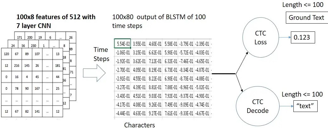
The CTC loss function is beneficial when the length of the input and output sequences are different, such as in the case of handwritten sentence recognition, where the length of the handwritten text in the image may be different from the length of the transcribed text.

The CTC loss function is based on a "blank" symbol, a special symbol that can be inserted between characters in the output sequence. The blank symbol is used to align the input and output sequences and allows the model to predict characters in the correct order, even if there are skips or repetitions in the input sequence.

Prerequisites:

Before we begin, you will need to have the following software installed:

• Python 3;
• TensorFlow (We will be using version 2.10 in this tutorial);
• mltu==0.1.7

Model preparation and Dataset:

TensorFlow is a Google-created, open-source system for performing machine learning tasks. It is widely used for training and deploying machine learning models and has many built-in tools and libraries for tasks such as image recognition, natural language processing, and more.

The first step in using TensorFlow and CTC loss for handwritten sentence recognition is to collect a dataset of handwritten sentences. This dataset should include a variety of handwriting styles and should be large enough to train a machine-learning model.

For this tutorial, I used IAM Dataset, which we must download manually from Handwriting Database. There is one downside, we must sign-up to download it, and I couldn't find a link to download it without registering. 

After downloading this Dataset (data/sentences.tgz), zip it in Datasets/IAM_Sentences folder. Also, you will need to download annotations (data/ascii.tgz) and zip it to the exact location. 

After doing so, we need to prepare the Dataset; this means we need to generate an exact path to the image with appropriate annotation. To do so, I wrote an iterative loop:

sentences_txt_path = stow.join('Datasets', 'IAM_Sentences', 'ascii', 'sentences.txt')
sentences_folder_path = stow.join('Datasets', 'IAM_Sentences', 'sentences')

dataset, vocab, max_len = [], set(), 0
words = open(sentences_txt_path, "r").readlines()
for line in tqdm(words):
    if line.startswith("#"):
        continue

    line_split = line.split(" ")
    if line_split[2] == "err":
        continue

    folder1 = line_split[0][:3]
    folder2 = line_split[0][:8]
    file_name = line_split[0] + ".png"
    label = line_split[-1].rstrip('\n')

    # recplace '|' with ' ' in label
    label = label.replace('|', ' ')

    rel_path = stow.join(sentences_folder_path, folder1, folder2, file_name)
    if not stow.exists(rel_path):
        continue

    dataset.append([rel_path, label])
    vocab.update(list(label))
    max_len = max(max_len, len(label))

This code is used to prepare a dataset for a machine-learning model. The Dataset consists of images of handwritten text and the corresponding text that is written in those images. The code first specifies the location of the text file and the folder where the images are stored. Then, it creates three empty variables, Dataset, vocab, and max_len. The code then opens the text file and reads all the lines. For each line in the text file, the code checks if the line starts with "#" or if the third word in the line is "err"; if so, it skips the line. If not, it takes the first three letters and the first eight letters of the first word in the line and uses them to create the folder path where the image is stored. It also creates a file name by adding ".png" to the first word. It also takes the last word in the line, which is the text written in the image, and removes the newline character at the end. Finally, the code adds the image path and the label to the Dataset and adds all the characters in the label to the vocab. It also keeps track of the most extended label in the Dataset so far.

Here are a few images from the dataset:

And these are only a few examples of thousands!

We know that when we want to get a robust and accurate machine learning model, the more data we have better it is, but for simplicity reasons, I chose only the IAM dataset. Many open-source datasets can be used for training and evaluating handwritten sentence recognition models, including:

• IAM: The IAM dataset is a collection of handwritten text images provided by the Institute of Document Analysis and Pattern Recognition at the University of Basel. The Dataset consists of 1,539 pages of handwritten text in English, German, and French and contains over 6,000 lines of text. It has been widely used in machine learning and computer vision research;
• Bentham: The Bentham dataset is a collection of manuscripts written by the English philosopher, jurist, and social reformer Jeremy Bentham. It contains over 600 manuscripts and is divided into four categories: political works, legal works, psychological works, and miscellaneous works. The manuscripts range from short notebooks to bound volumes, and each includes an introduction, a list of contents, and detailed descriptions of the individual works;
• Rimes: Rimes is a large dataset of handwritten text in French, with over 1 million annotated words. It was designed for handwriting recognition research, including isolated characters and lines of text. The Dataset contains varying levels of difficulty in terms of letter size, writing style, and handwriting quality;
• Washington: The Washington dataset is a collection of 1,800 images of handwritten English text. It was created for handwriting recognition and machine learning research and contains isolated characters and text lines. The Dataset is divided into three categories: easy, medium, and challenging, with varying difficulty levels;
• Saint Gall: The Saint Gall dataset is a collection of 6,000 images of the handwritten Latin text from the 8th to the 10th centuries. This Dataset is a valuable resource for historical document analysis and handwriting recognition, as it is composed of manuscripts preserved for centuries. It has also been used for training natural language processing models.

You could use these different datasets to expand the training set.

Next, the Dataset must be preprocessed and prepared for use in the model. This can involve tasks such as reading images, converting the images of handwritten sentences into a suitable format, indexing labels, padding labels, and dividing the Dataset into training and testing sets. Precisely in the same way as before, I am doing these steps with a custom DataProvider object:

# Create a data provider for the dataset
data_provider = DataProvider(
    dataset=dataset,
    skip_validation=True,
    batch_size=configs.batch_size,
    data_preprocessors=[ImageReader()],
    transformers=[
        ImageResizer(configs.width, configs.height, keep_aspect_ratio=True),
        LabelIndexer(configs.vocab),
        LabelPadding(max_word_length=configs.max_text_length, padding_value=len(configs.vocab)),
        ],
)

# Split the dataset into training and validation sets
train_data_provider, val_data_provider = data_provider.split(split = 0.9)

Also, when training machine learning models, it's crucial to apply data augmentation techniques to achieve better training results. In this tutorial, I am using RandomBrightness, RandomErodeDilate, and RandomSharpen augmentors to the training data provider object:

# Augment training data with random brightness, rotation and erode/dilate
train_data_provider.augmentors = [
    RandomBrightness(), 
    RandomErodeDilate(),
    RandomSharpen(),
    ]

Defining model architecture:

Once the Dataset is prepared, the next step is to design and train a machine-learning model using TensorFlow and CTC loss. This involves selecting an appropriate model architecture and choosing hyperparameters such as the learning rate and batch size. Here are a few recommendations when creating the model:

1. We define the input and output layers: The input layer of the model should be a 4D tensor with dimensions [batch size, width, height, channels], where the batch size is the number of images in a batch, width and height are the dimensions of the images, and channels is the number of color channels in the images (1 for grayscale, 3 for RGB);
2. Add the CNN layers: The CNN layers of the model should be responsible for extracting features from the images. A typical architecture for the CNN layers is to use a combination of convolutional, pooling, and fully-connected (dense) layers;
3. Add the RNN layers: The RNN layers of the model should be responsible for processing the sequence of features and predicting the characters in the text. A common type of RNN to use for this task is a long short-term memory (LSTM) network;
4. Finally, we compile the model: Once the CNN and RNN layers have been defined, the model can be compiled using the CTC loss function and an optimizer such as Adam.

Here is the basic architecture of the model used in this tutorial:

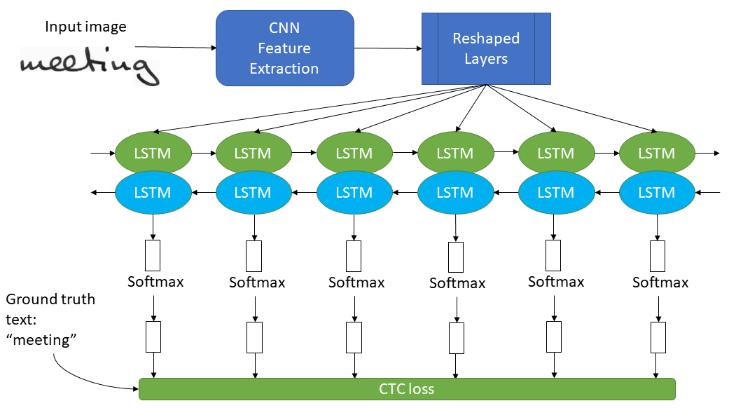
When we have our model, it can then be trained on the training set using an optimization algorithm, such as Adam. During training, the model will make predictions on the input data. Utilizing the CTC loss function, the model will update to reduce the disparity between the estimated values and the actual labels.

We will use the following code to create the model, compile it, define the optimizer, loss, metrics, and callbacks and initiate the training process:

# Creating TensorFlow model architecture
model = train_model(
    input_dim = (configs.height, configs.width, 3),
    output_dim = len(configs.vocab),
)

# Compile the model and print summary
model.compile(
    optimizer=tf.keras.optimizers.Adam(learning_rate=configs.learning_rate), 
    loss=CTCloss(), 
    metrics=[
        CERMetric(vocabulary=configs.vocab),
        WERMetric(vocabulary=configs.vocab)
        ],
)
model.summary(line_length=110)

# Define callbacks
earlystopper = EarlyStopping(monitor='val_CER', patience=20, verbose=1, mode='min')
checkpoint = ModelCheckpoint(f"{configs.model_path}/model.h5", monitor='val_CER', verbose=1, save_best_only=True, mode='min')
trainLogger = TrainLogger(configs.model_path)
tb_callback = TensorBoard(f'{configs.model_path}/logs', update_freq=1)
reduceLROnPlat = ReduceLROnPlateau(monitor='val_CER', factor=0.9, min_delta=1e-10, patience=5, verbose=1, mode='auto')
model2onnx = Model2onnx(f"{configs.model_path}/model.h5")

# Train the model
model.fit(
    train_data_provider,
    validation_data=val_data_provider,
    epochs=configs.train_epochs,
    callbacks=[earlystopper, checkpoint, trainLogger, reduceLROnPlat, tb_callback, model2onnx],
    workers=configs.train_workers
)

Training the model:

Several metrics can be used to evaluate the training performance of a handwritten sentence recognition model. But two of them are the most popular for tasks related to text extraction. We can check them out with the help of a TensorBoard callback (tensorboard --logdir Models/04_sentence_recognition/202301131202/logs) used while training the model.

The CER, or Character Error Rate, is a metric used to evaluate the performance of a handwritten sentence recognition model. It is calculated as the number of characters that are incorrectly recognized by the model, divided by the total number of characters in the ground truth text. In the following image, we can see the training (orange color) curve and blue (validation) curves:

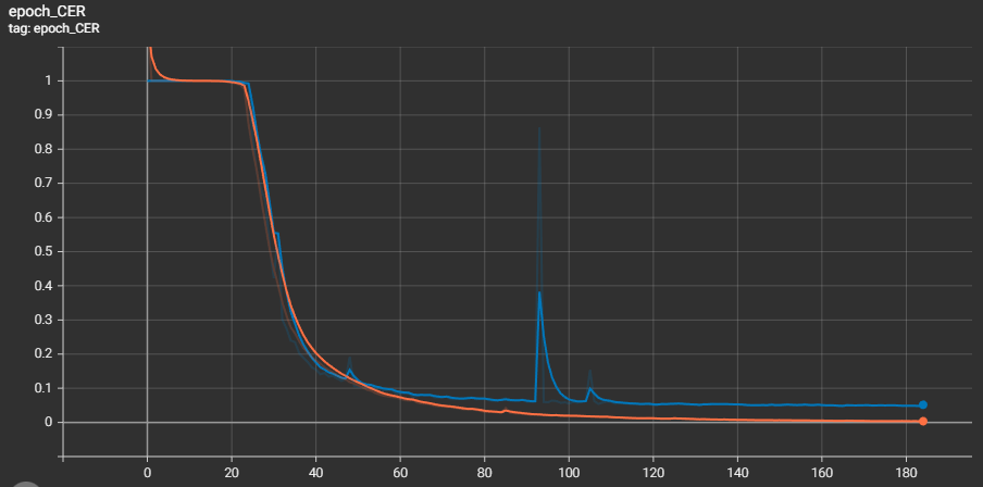
We can see a massive difference between training and validation curves, but the goal of this tutorial is not to train the best Hand Written Sentence recognition model. 

The WER, or Word Error Rate, is another metric used to evaluate the performance of a handwritten sentence recognition model. It is calculated as the number of words incorrectly recognized by the model divided by the total number of words in the ground truth text. We have a similar graph as we had for CER:

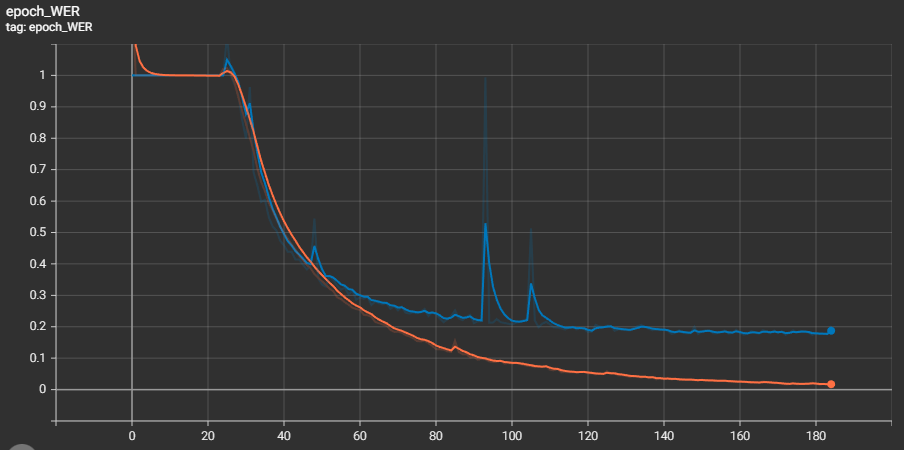
This Word Error Rate graph shows an even bigger difference between training and validation data. But the goal was to see overall improvement while training, which is what we did!

CER and WER metrics are primarily used metrics in OCR systems and help evaluate the accuracy of a model.

Testing the model:

Once the model has been trained, it is ready to be tested on new data. To test the model, you will need to:

1. Preprocess the test data: The test data should be preprocessed in the same way as the training data.
2. Evaluate the model on the test data: The model's performance on the test data can be evaluated using the CTC loss and any additional metrics that you defined during training.

But there is no point testing it out while we already received CER and WER graphs above from training and evaluation processes. So let's run inference on an already trained model that was converter to .ONNX model. To do so, I wrote a script:

# inferenceModel.py
import cv2
import typing
import numpy as np

from mltu.inferenceModel import OnnxInferenceModel
from mltu.utils.text_utils import ctc_decoder, get_cer, get_wer
from mltu.transformers import ImageResizer

class ImageToWordModel(OnnxInferenceModel):
    def __init__(self, char_list: typing.Union[str, list], *args, **kwargs):
        super().__init__(*args, **kwargs)
        self.char_list = char_list

    def predict(self, image: np.ndarray):
        image = ImageResizer.resize_maintaining_aspect_ratio(image, *self.input_shape[:2][::-1])

        image_pred = np.expand_dims(image, axis=0).astype(np.float32)

        preds = self.model.run(None, {self.input_name: image_pred})[0]

        text = ctc_decoder(preds, self.char_list)[0]

        return text

if __name__ == "__main__":
    import pandas as pd
    from tqdm import tqdm
    from mltu.configs import BaseModelConfigs

    configs = BaseModelConfigs.load("Models/04_sentence_recognition/202301131202/configs.yaml")

    model = ImageToWordModel(model_path=configs.model_path, char_list=configs.vocab)

    df = pd.read_csv("Models/04_sentence_recognition/202301131202/val.csv").values.tolist()

    accum_cer, accum_wer = [], []
    for image_path, label in tqdm(df):
        image = cv2.imread(image_path)

        prediction_text = model.predict(image)

        cer = get_cer(prediction_text, label)
        wer = get_wer(prediction_text, label)
        print("Image: ", image_path)
        print("Label:", label)
        print("Prediction: ", prediction_text)
        print(f"CER: {cer}; WER: {wer}")

        accum_cer.append(cer)
        accum_wer.append(wer)

        cv2.imshow(prediction_text, image)
        cv2.waitKey(0)
        cv2.destroyAllWindows()

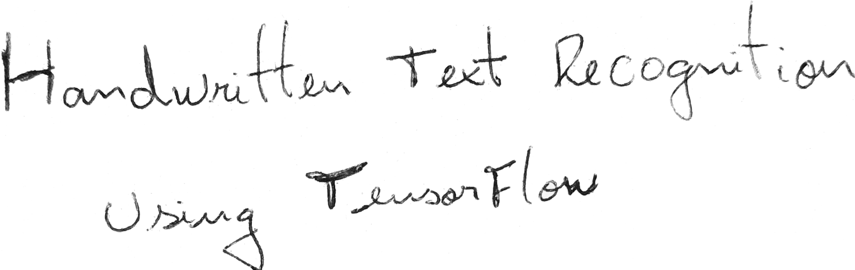
    print(f"Average CER: {np.average(accum_cer)}, Average WER: {np.average(accum_wer)}")

Here are several image and prediction results from our validation data:

Label: "of Betti's writing without over-emphasizing"

Prediction:  "of Bettis writing without over-emphasiging"

CER: 0.046511627906976744; WER: 0.4

Label: "has made it difficult for corporations to achieve"

Prediction:  "has mad it dificult for corporations to active"

CER: 0.061224489795918366; WER: 0.375

Label: "food scheme ."

Prediction:  "food scheme ."

CER: 0.07692307692307693; WER: 0.3333333333333333

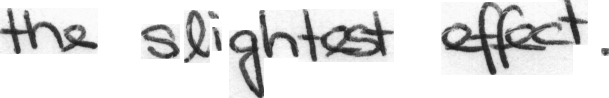
Label: "the slightest effect ."

Prediction:  "the slightest effect ."

CER: 0.0; WER: 0.0

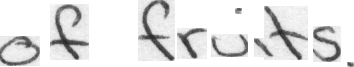
Label: "of fruits ."

Prediction:  "of friits ."

CER: 0.09090909090909091; WER: 0.3333333333333333

Label: "conventional remedies to which he had been subjected"

Prediction:  "conventional remedies to which he had been subjeded"

CER: 0.038461538461538464; WER: 0.125

From the above results, we can clearly say that our model is making the right predictions. Of course, it makes minor mistakes, but it wasn't our goal to make it perfect. To make it even better, you can play with different architectures, add more training data, and apply more data augmentation techniques. There is a lot of room for improvement!

Conclusion:

This tutorial covered building a model for handwritten sentence recognition using TensorFlow and the CTC loss function. We discussed the challenges and use cases of handwritten sentence recognition and looked at various methods and techniques for solving this problem. We also discussed the metrics that can be used to evaluate the performance of a model and introduced several datasets that can be used for training and evaluation. Finally, we looked at ways to improve the model's performance and discussed the importance of preprocessing the data and choosing the exemplary model architecture.

Building a model for handwritten sentence recognition using TensorFlow is a fun and exciting challenge!

The trained model used in this tutorial can be downloaded from this link.

Complete tutorial code on GitHub.