In the previous tutorial, we got familiar with Transformers. What are they, and what advantages and limitations do they bring. Also, we started implementing it in TensorFlow by going step-by-step. So, we implemented the PositionalEmbedding layer. Here is the architecture of Transformers:

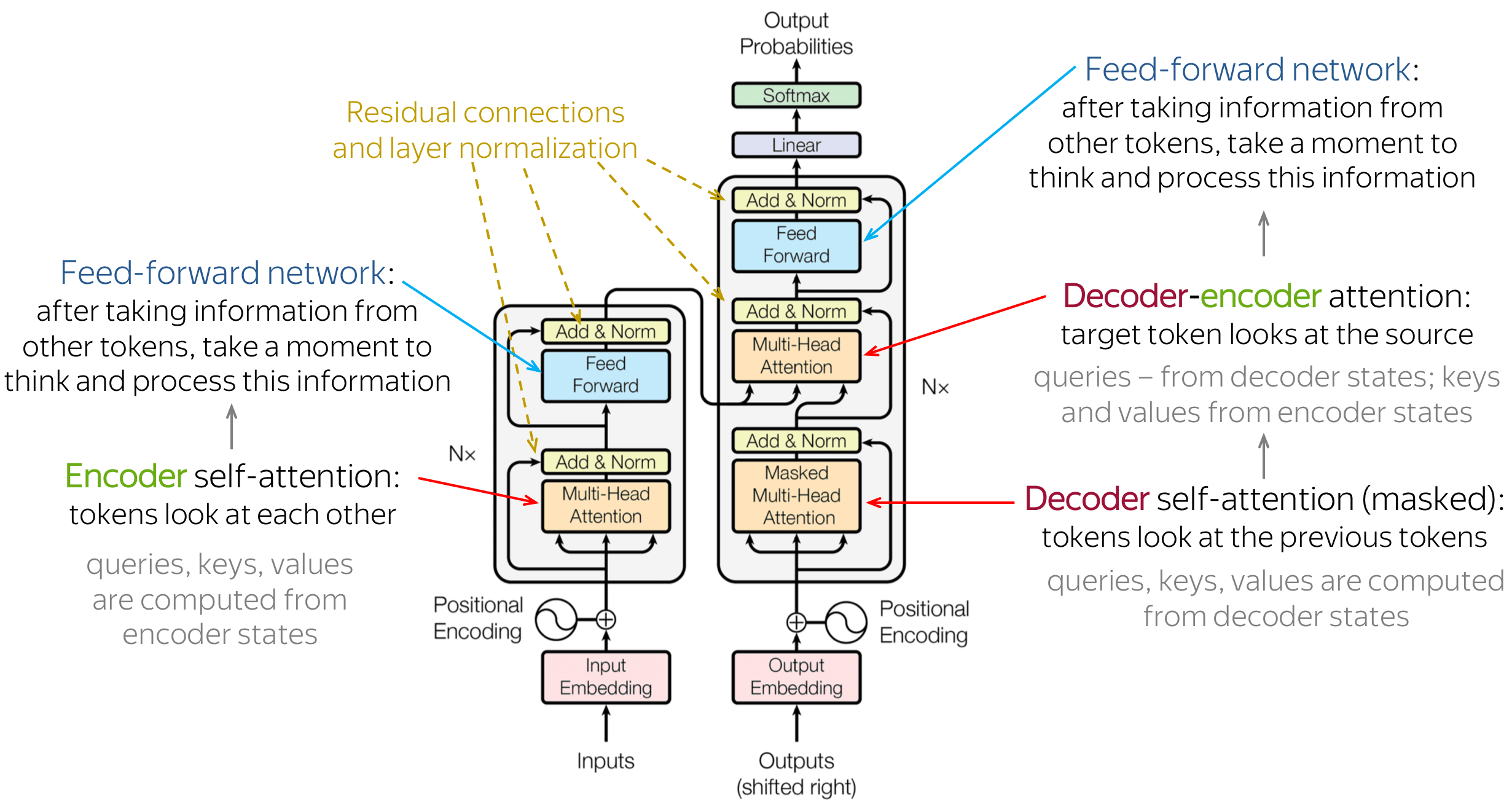In this tutorial part, we'll implement the following:

• Add & Norm layer;
• BaseAttention layer;
• CrossAttention layer;
• GlobalSelfAttention layer;
• CausalSelfAttention layer;
• FeedForward layer.

While implementing each of these layers, we'll better understand the Transformer Architecture and these layers purpose.

Add & Norm:

If you pay attention to Transformer architecture, you may notice an Add & Norm layer after each attention layer. This layer is responsible for adding the residual connection and applying layer normalization:

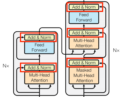
The Transformer model utilizes "Add & Norm" blocks to facilitate efficient training. These blocks incorporate two essential components: a residual connection and a LayerNormalization layer.

The residual connection establishes a direct path for the gradient, ensuring that vectors are updated rather than entirely replaced by the attention layers. This helps with gradient flow during training. On the other hand, the LayerNormalization layer maintains a reasonable scale for the outputs, enhancing the stability and performance of the model.

The Transformer model has strategically placed "Add & Norm" blocks, with corresponding custom layer classes defined to handle them. To ensure proper propagation of Keras masks, the implementation employs the "Add" layer instead of the "+" operator alone, which does not handle mask propagation.

In summary, the "Add & Norm" blocks are crucial in the Transformer model, ensuring effective training by incorporating residual connections and LayerNormalization. Custom layer classes are utilized to handle these blocks, with the "Add" layer addressing mask propagation within the implementation.

We'll not create a separate layer for this addition and normalization functionality. Instead, we'll create a BaseAttention and FeedForward layer that will handle these operations for us.

BaseAttention layer:

The attention mechanism is the core component of the Transformer model. It enables the model to focus on the relevant parts of the input sequence when processing each token. This is achieved by calculating the attention weights between each token's query and key vectors in the sequence. The attention weights are then multiplied by the value vectors to obtain the context vector, which is the output of the attention layer.

We'll implement all the attention layers used in the Transformer model. First, we'll create a base class for all attention layers:

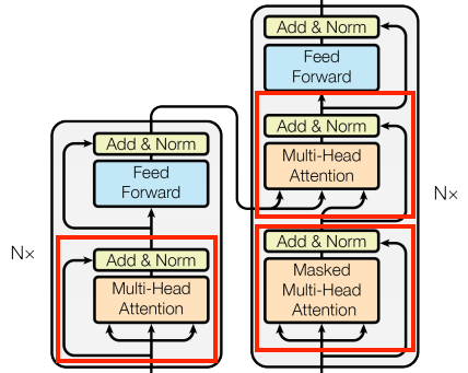
These are all identical except for how the attention is configured. Each contains a layers.MultiHeadAttention, a layers.LayerNormalization, and a layers.Add layers. We can create a base class that takes care of all of this. The only thing we need to do later is to implement the call method.

We can begin by creating a basic class that includes the necessary component layers to implement the attention layers. Each specific use case can then be implemented as a subclass of this base class. Although this approach requires writing a bit more code, it helps maintain clarity and ensures that the purpose of each subclass remains apparent:

class BaseAttention(tf.keras.layers.Layer):
    """
    Base class for all attention layers. It contains the common functionality of all attention layers.
    This layer contains a MultiHeadAttention layer, a LayerNormalization layer and an Add layer.
    It is used as a base class for the GlobalSelfAttention, CausalSelfAttention and CrossAttention layers.
    And it is not intended to be used directly.

    Methods:
        call: Performs the forward pass of the layer.

    Attributes:
        mha (tf.keras.layers.MultiHeadAttention): The MultiHeadAttention layer.
        layernorm (tf.keras.layers.LayerNormalization): The LayerNormalization layer.
        add (tf.keras.layers.Add): The Add layer.
    """
    def __init__(self, **kwargs: dict):
        """ Constructor of the BaseAttention layer.
        
        Args:
            **kwargs: Additional keyword arguments that are passed to the MultiHeadAttention layer, e. g. 
                        num_heads (number of heads), key_dim (dimensionality of the key space), etc.
        """
        super().__init__()
        self.mha = tf.keras.layers.MultiHeadAttention(**kwargs)
        self.layernorm = tf.keras.layers.LayerNormalization()
        self.add = tf.keras.layers.Add()

Within the class, there are three essential layers: tf.keras.layers.MultiHeadAttention, tf.keras.layers.LayerNormalization, and tf.keras.layers.Add:

• The MultiHeadAttention layer computes the attention weights, which determine the relevance or importance of different parts of the input and output sequences;
• The LayerNormalization layer normalizes the layer's activations, ensuring they have a consistent scale across batch and feature dimensions;
• The Add layer incorporates a residual connection. It adds the output of the MultiHeadAttention layer to the original input sequence, allowing the model to retain information from the initial input while incorporating the attention-based updates.

We can reuse the code and easily create different attention mechanisms by creating a base class that includes these layers. This is achieved by inheriting from the base class and specifying the unique implementation details for each specific attention mechanism. This approach aids in maintaining code organization and clarity throughout the implementation.

But still, you may ask, how it works?

An attention layer has two main inputs: the query and context sequences. The query sequence represents the sequence we focus on, while the context sequence is the one we seek information from. The output of the attention layer has the same shape as the query sequence.

The operation of an attention layer can be likened to a dictionary lookup but with some distinct characteristics. Like a regular dictionary, a query is used to search for relevant information represented by keys and values. In a standard dictionary, an exact match between the query and a key is necessary to retrieve the corresponding value. However, in an attention layer, the match does not need to be exact; it can be fuzzy or approximate.

For example, if we searched for the key "species" in the dictionary {'color': 'blue', 'age': 22, 'type': 'pickup'}, the best match might be the value "pickup" even though the query and key don't match perfectly.

In an attention layer, multiple values are combined based on their similarity to the query, rather than returning a single value. Each component (query, key, and value) in the attention layer is represented as vectors. Instead of using a traditional dictionary lookup, the attention layer calculates an attention score by comparing the query and key vectors. The values are then combined by taking a weighted average, where the attention scores determine the weights.

In the context of natural language processing (NLP), the query sequence can provide a query vector at each position. In contrast, the context sequence serves as the dictionary, with key and value vectors at each position. Before using the input vectors, the layers.MultiHeadAttention layer employs layers.Dense layers to project these vectors.

So now, let's use this class to create other attention layers. We will create:

• The cross-attention layer: Decoder-encoder attention;
• The global self-attention layer: Encoder self-attention;
• The causal self-attention layer: Decoder self-attention.

CrossAttention layer

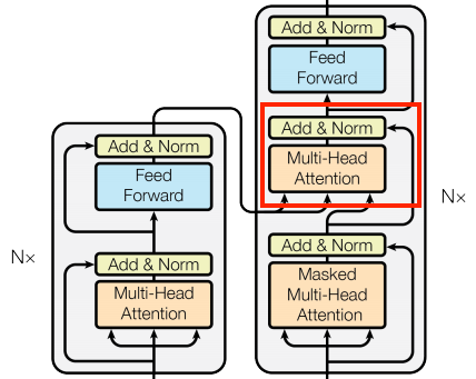
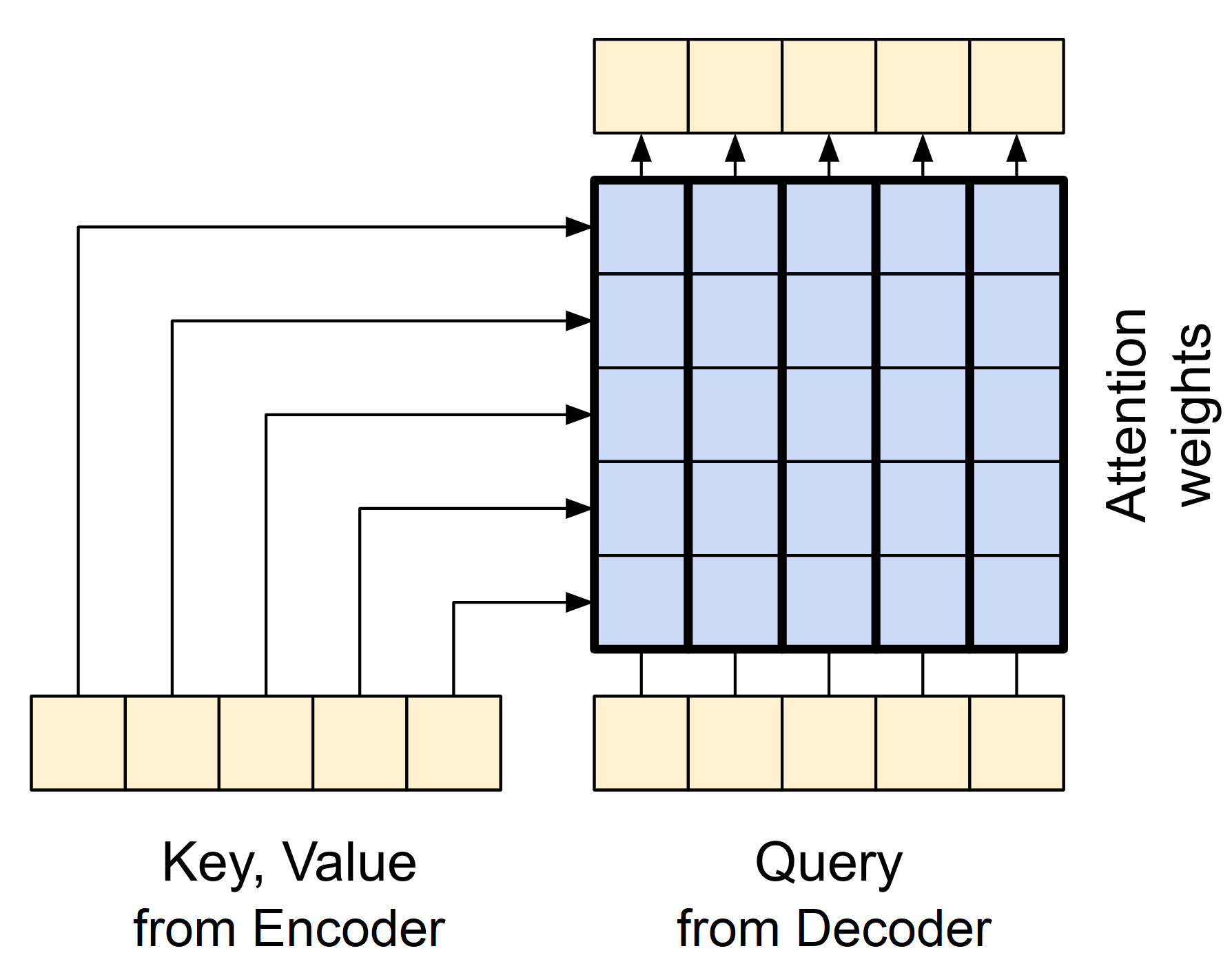
The query vectors are taken from the decoder, while the key and value vectors are taken from the encoder. Using this method, the decoder can concentrate on the essential sections of the input sequence while producing a token for each position.

When implementing this layer, we pass the target (expected Transformer results) sequence x as the query and the context (inputs to the Encoder layer) sequence as the value and key:

class CrossAttention(BaseAttention):
    """
    A class that implements the cross-attention layer by inheriting from the BaseAttention class.
    This layer is used to process two different sequences and attends to the context sequence while processing the query sequence.

    Methods:
        call: Performs the forward pass of the layer.    

    Attributes:
        mha (tf.keras.layers.MultiHeadAttention): The MultiHeadAttention layer.
        layernorm (tf.keras.layers.LayerNormalization): The LayerNormalization layer.
        add (tf.keras.layers.Add): The Add layer.
    """
    def call(self, x: tf.Tensor, context: tf.Tensor) -> tf.Tensor:
        """
        The call function that performs the cross-attention operation.

        Args:
            x (tf.Tensor): The query (expected Transformer results) sequence of shape (batch_size, seq_length, d_model).
            context (tf.Tensor): The context (inputs to the Encoder layer) sequence of shape (batch_size, seq_length, d_model).

        Returns:
            tf.Tensor: The output sequence of shape (batch_size, seq_length, d_model).
        """
        attn_output, attn_scores = self.mha(query=x, key=context, value=context, return_attention_scores=True)

        # Cache the attention scores for plotting later.
        self.last_attn_scores = attn_scores

        x = self.add([x, attn_output])
        x = self.layernorm(x)

        return x

Let's test this CrossAttention layer. To do so, we'll create a simulated random data that we pass through the PositionalEncoding layer and then to the CrossAttention layer:

encoder_vocab_size = 1000
decoder_vocab_size = 1100
d_model = 512

encoder_embedding_layer = PositionalEmbedding(vocab_size, d_model)
decoder_embedding_layer = PositionalEmbedding(vocab_size, d_model)

random_encoder_input = np.random.randint(0, encoder_vocab_size, size=(1, 100))
random_decoder_input = np.random.randint(0, decoder_vocab_size, size=(1, 110))

encoder_embeddings = encoder_embedding_layer(random_encoder_input)
decoder_embeddings = decoder_embedding_layer(random_decoder_input)

print("encoder_embeddings shape", encoder_embeddings.shape)
print("decoder_embeddings shape", decoder_embeddings.shape)

cross_attention_layer = CrossAttention(num_heads=2, key_dim=512)
cross_attention_output = cross_attention_layer(decoder_embeddings, encoder_embeddings)

print("cross_attention_output shape", cross_attention_output.shape)

We should get the following output:

encoder_embeddings shape (1, 100, 512)
decoder_embeddings shape (1, 110, 512)
cross_attention_output shape (1, 110, 512)

You can see that the output shape from the CrossAttention layer is the same as the decoder embedding shape. This is because the output of the cross-attention layer is the same as the query sequence, which is the target sequence in this case. The simplified diagram below illustrates the information flow in the cross-attention layer:

GlobalSelfAttention layer

The GlobalSelfAttention layer is responsible for processing the context (encoder input) sequence and propagating information along its length:

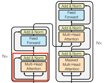
The GlobalSelfAttention layer allows each element in a sequence to easily access all other elements with minimal effort, and all results can be calculated simultaneously.

To implement this layer, it is crucial to supply the target sequence, x, as the query and value arguments to the mha layer.

class GlobalSelfAttention(BaseAttention):
    """
    A class that implements the global self-attention layer by inheriting from the BaseAttention class.
    This layer is used to process a single sequence and attends to all the tokens in the sequence.

    Methods:
        call: Performs the forward pass of the layer.

    Attributes:
        mha (tf.keras.layers.MultiHeadAttention): The MultiHeadAttention layer.
        layernorm (tf.keras.layers.LayerNormalization): The LayerNormalization layer.
        add (tf.keras.layers.Add): The Add layer.
    """
    def call(self, x: tf.Tensor) -> tf.Tensor:
        """
        The call function that performs the global self-attention operation.

        Args:
            x (tf.Tensor): The input sequence of shape (batch_size, seq_length, d_model).

        Returns:
            tf.Tensor: The output sequence of shape (batch_size, seq_length, d_model).
        """
        attn_output = self.mha(query=x, value=x, key=x)
        x = self.add([x, attn_output])
        x = self.layernorm(x)
        return x

The Multi-Head Attention (MHA) mechanism calculates a weighted average of values based on the similarity between queries and keys. The attention scores assigned to each value determine its importance.

In simpler terms, the MHA learns to focus on different parts of the input sequence, allowing the model to extract relevant information for a specific task. In the case of GlobalSelfAttention, where the input sequence serves as both the query and key, it captures the relationships between each position and all other positions in the sequence. We can visualize this process as follows:

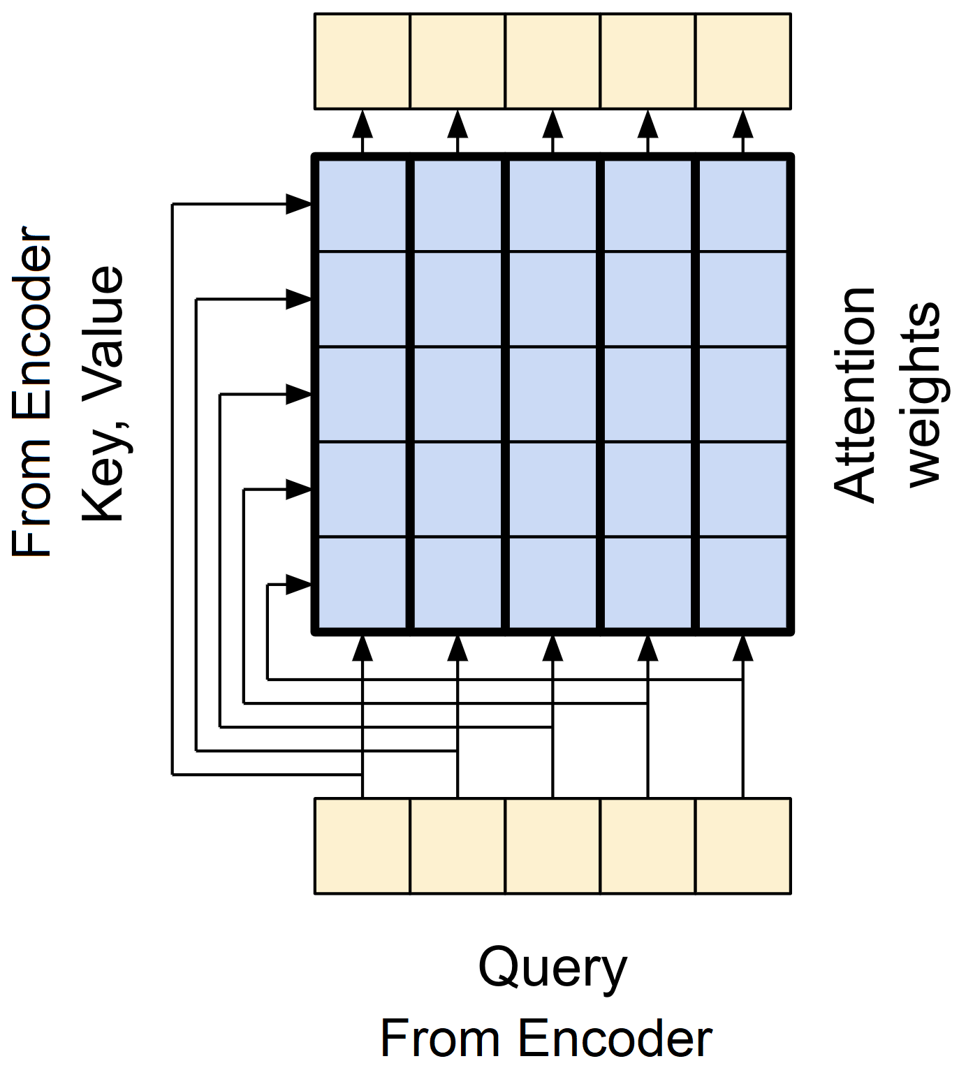
Subsequently, the output of the MHA is added to the original input. This result is passed through layer normalization, stabilizing the training process and enhancing the model's performance. Ultimately, this normalized output represents the final output of the attention layer.

Let's test it out:

encoder_vocab_size = 1000
d_model = 512

encoder_embedding_layer = PositionalEmbedding(vocab_size, d_model)

random_encoder_input = np.random.randint(0, encoder_vocab_size, size=(1, 100))

encoder_embeddings = encoder_embedding_layer(random_encoder_input)

print("encoder_embeddings shape", encoder_embeddings.shape)

cross_attention_layer = GlobalSelfAttention(num_heads=2, key_dim=512)
cross_attention_output = cross_attention_layer(encoder_embeddings)

print("global_self_attention_output shape", cross_attention_output.shape)

We should see the following output:

encoder_embeddings shape (1, 100, 512)
global_self_attention_output shape (1, 100, 512)

CausalSelfAttention layer

The CausalSelfAttention layer is responsible for processing the target (decoder input) sequence and propagating information along its length:

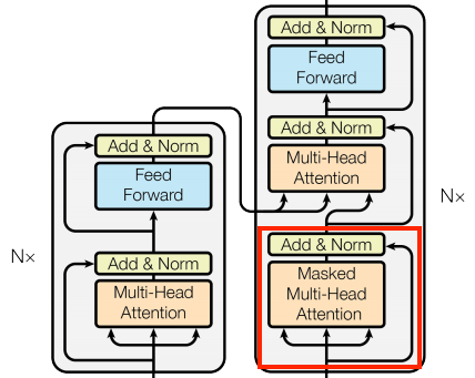
The CausalSelfAttention layer operates similarly to the GlobalSelfAttention layer, allowing each sequence element to access all other sequence elements with minimal operations and resulting in parallel computation of all outputs.

But the CausalSelfAttention layer differs from GlobalSelfAttention because it prevents leftward information flow in the decoder. Masking is crucial in this process, as it prevents the model from attending to future tokens during training. This masking process is illustrated in the diagram below:

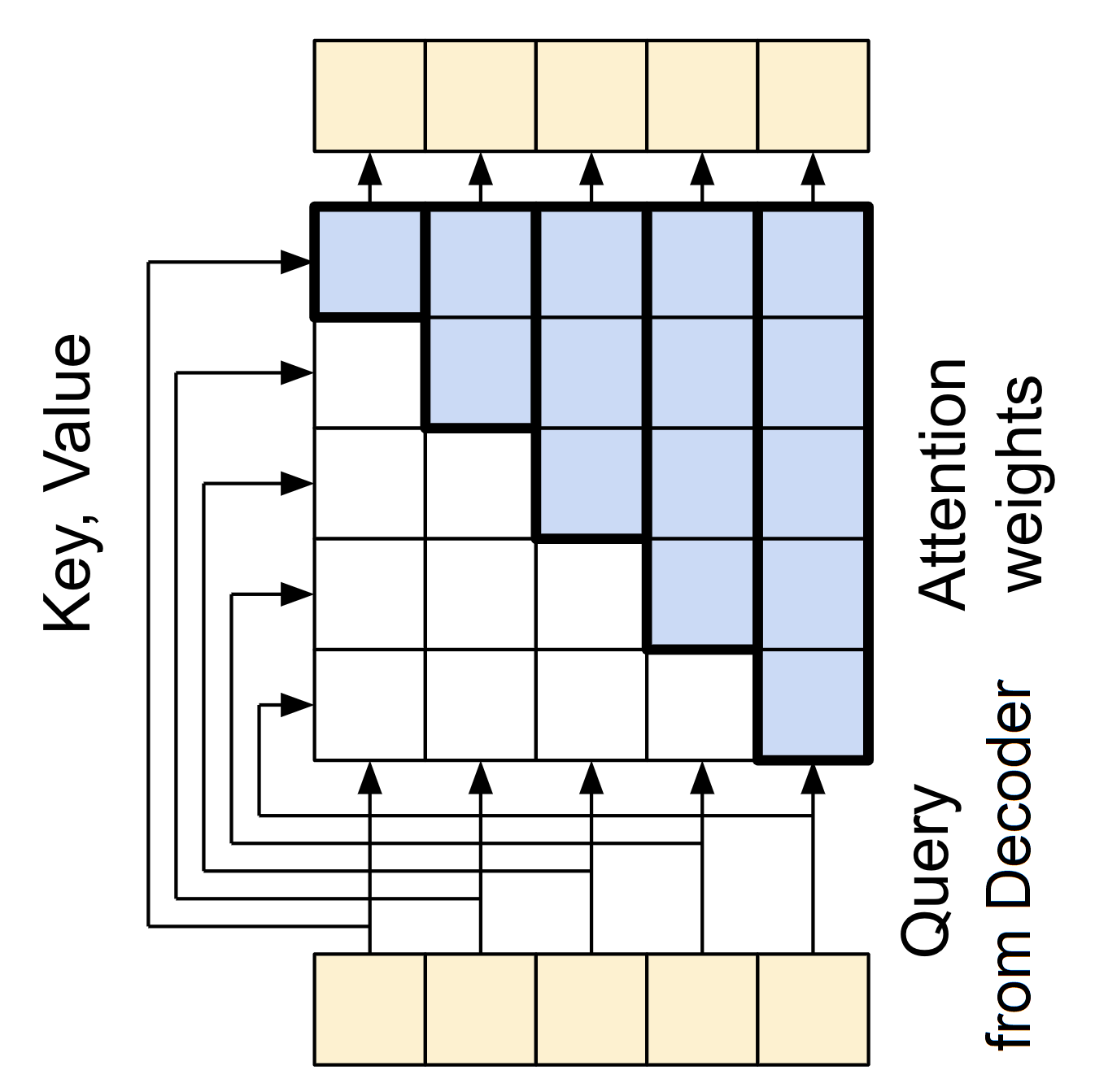The causal mask prevents each location from accessing any locations that come after it, ensuring that it only has access to those that come before it. Let's write this layer in code:

class CausalSelfAttention(BaseAttention):
    """
    Call self attention on the input sequence, ensuring that each position in the 
    output depends only on previous positions (i.e. a causal model).

    Methods:
        call: Performs the forward pass of the layer.

    Attributes:
        mha (tf.keras.layers.MultiHeadAttention): The MultiHeadAttention layer.
        layernorm (tf.keras.layers.LayerNormalization): The LayerNormalization layer.
        add (tf.keras.layers.Add): The Add layer.
    """
    def call(self, x: tf.Tensor) -> tf.Tensor:
        """
        The call function that performs the causal self-attention operation.
        
        Args:
            x (tf.Tensor): The input sequence of shape (batch_size, seq_length, d_model).

        Returns:
            tf.Tensor: The output sequence of shape (batch_size, seq_length, d_model).
        """
        attn_output = self.mha(query=x, value=x, key=x, use_causal_mask = True)
        x = self.add([x, attn_output])
        x = self.layernorm(x)
        return x

You may notice that the CausalSelfAttention layer is very similar to the GlobalSelfAttention layer. The only difference is that the CausalSelfAttention layer uses a causal mask to prevent the decoder from attending to future tokens during training.

As before, let's test this CausalSelfAttention layer. To do so, we'll create a simulated random data that we pass through the PositionalEncoding layer and then to the CausalSelfAttention layer:

decoder_vocab_size = 1100
d_model = 512

decoder_embedding_layer = PositionalEmbedding(vocab_size, d_model)

random_decoder_input = np.random.randint(0, decoder_vocab_size, size=(1, 110))

decoder_embeddings = decoder_embedding_layer(random_decoder_input)

print("decoder_embeddings shape", decoder_embeddings.shape)

causal_self_attention_layer = CausalSelfAttention(num_heads=2, key_dim=512)
causal_self_attention_output = causal_self_attention_layer(decoder_embeddings)

print("causal_self_attention_output shape", causal_self_attention_output.shape)

out1 = causal_self_attention_layer(decoder_embedding_layer(random_decoder_input[:, :50])) # Only the first 50 tokens beffore applying the embedding layer
out2 = causal_self_attention_layer(decoder_embedding_layer(random_decoder_input)[:, :50]) # Only the first 50 tokens after applying the embedding layer

diff = tf.reduce_max(tf.abs(out1 - out2)).numpy()

print("Difference between the two outputs:", diff)

You should see the following output:

decoder_embeddings shape (1, 110, 512)
causal_self_attention_output shape (1, 110, 512)
Difference between the two outputs: 0.0

It doesn't really matter whether you trim the early sequence elements before or after applying the embedding layer, as the output for those elements is not dependent on the later ones. In essence, there is no difference between these two approaches.

FeedForward layer

Looking closer at the encoder and decoder layers, we can see that there is a FeedForward layer after each attention layer:

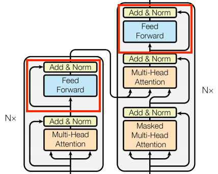
The FeedForward layer comprises two dense layers that are individually and uniformly applied to every position. The FeedForward layer is primarily used to transform the representation of the input sequence into a more suitable form for the task at hand. This is achieved by applying a linear transformation followed by a non-linear activation function. The output of the FeedForward layer has the same shape as the input, which is then added to the original input.

Let's implement this layer:

class FeedForward(tf.keras.layers.Layer):
    """
    A class that implements the feed-forward layer.

    Methods:
        call: Performs the forward pass of the layer.

    Attributes:
        seq (tf.keras.Sequential): The sequential layer that contains the feed-forward layers. It applies the two feed-forward layers and the dropout layer.
        add (tf.keras.layers.Add): The Add layer.
        layer_norm (tf.keras.layers.LayerNormalization): The LayerNormalization layer.
    """
    def __init__(self, d_model: int, dff: int, dropout_rate: float=0.1):
        """
        Constructor of the FeedForward layer.

        Args:
            d_model (int): The dimensionality of the model.
            dff (int): The dimensionality of the feed-forward layer.
            dropout_rate (float): The dropout rate.
        """
        super().__init__()
        self.seq = tf.keras.Sequential([
            tf.keras.layers.Dense(dff, activation='relu'),
            tf.keras.layers.Dense(d_model),
            tf.keras.layers.Dropout(dropout_rate)
        ])
        self.add = tf.keras.layers.Add()
        self.layer_norm = tf.keras.layers.LayerNormalization()

    def call(self, x: tf.Tensor) -> tf.Tensor:
        """
        The call function that performs the feed-forward operation. 

        Args:
            x (tf.Tensor): The input sequence of shape (batch_size, seq_length, d_model).

        Returns:
            tf.Tensor: The output sequence of shape (batch_size, seq_length, d_model).
        """
        x = self.add([x, self.seq(x)])
        x = self.layer_norm(x) 
        return x

Let's test the FeedForward layer. We will use the same random input as before. The output shape should be the same as the input shape.

encoder_vocab_size = 1000
d_model = 512

encoder_embedding_layer = PositionalEmbedding(vocab_size, d_model)

random_encoder_input = np.random.randint(0, encoder_vocab_size, size=(1, 100))

encoder_embeddings = encoder_embedding_layer(random_encoder_input)

print("encoder_embeddings shape", encoder_embeddings.shape)

feed_forward_layer = FeedForward(d_model, dff=2048)
feed_forward_output = feed_forward_layer(encoder_embeddings)

print("feed_forward_output shape", feed_forward_output.shape)

You should see the following output:

encoder_embeddings shape (1, 100, 512)
feed_forward_output shape (1, 100, 512)

Conclusion:

In this tutorial, we covered the most essential parts of the Transformer architecture. We understood the crucial difference between CrossAttention, GlobalSelfAttention, and CausalSelfAttention layers. Although we implemented each of these layers in TensorFlow and understood what the input and outputs are.

Wrapping up, we:

🎯 Understood the main blocks of the Transformer;

🎓 Implemented Attention layers and Understood their Significance.

💡 Built a Custom "Add & Norm", "FeedForward", "BaseAttention" and other layers in TensorFlow.

💻 Tested these Layers with Random Input Sequences.

This tutorial is part of the Transformer series. It's crucial to understand this part to continue understanding how Transformers work. In the next tutorial, we'll use these layers to build an Encoder and Decoder for Transformer architecture.