TensorFlow Keras ResNet tutorial

Welcome to another tutorial! Now we will learn how to build very deep convolutional networks using Residual Networks (ResNets). This model was the winner of the ImageNet challenge in 2015. The fundamental breakthrough with ResNet was it allowed us to train extremely deep neural networks with 150+layers successfully. Before ResNet training, very deep Neural Networks were difficult due to the problem of vanishing gradients.

Deep networks are hard to train because of the vanishing gradient problem — as the gradient is back-propagated to earlier layers, repeated multiplication may make the gradient extremely small. However, increasing network depth does not work by simply stacking layers together. As a result, as the network goes deeper, its performance gets saturated or degrades rapidly.

In this tutorial, we will:

• Implement the basic building blocks of ResNets;
• Put together these building blocks to implement and train a state-of-the-art neural network for image classification.

Let's run the cell below to load the required packages:

import os
os.environ['CUDA_VISIBLE_DEVICES'] = '0'
import cv2
import numpy as np
from keras import layers
from keras.layers import Input, Add, Dense, Activation, ZeroPadding2D, BatchNormalization, Flatten, Conv2D, AveragePooling2D, MaxPooling2D
from keras.models import Model, load_model
from keras.initializers import glorot_uniform
from keras.utils import plot_model
from IPython.display import SVG
from keras.utils.vis_utils import model_to_dot
import keras.backend as K
import tensorflow as tf

ROWS = 64
COLS = 64
CHANNELS = 3
CLASSES = 2

def read_image(file_path):
    img = cv2.imread(file_path, cv2.IMREAD_COLOR)
    return cv2.resize(img, (ROWS, COLS), interpolation=cv2.INTER_CUBIC)

def prepare_data(images):
    m = len(images)
    X = np.zeros((m, ROWS, COLS, CHANNELS), dtype=np.uint8)
    y = np.zeros((1, m), dtype=np.uint8)
    for i, image_file in enumerate(images):
        X[i,:] = read_image(image_file)
        if 'dog' in image_file.lower():
            y[0, i] = 1
        elif 'cat' in image_file.lower():
            y[0, i] = 0
    return X, y

def convert_to_one_hot(Y, C):
    Y = np.eye(C)[Y.reshape(-1)].T
    return Y

TRAIN_DIR = 'Train_data/'
TEST_DIR = 'Test_data/'

train_images = [TRAIN_DIR+i for i in os.listdir(TRAIN_DIR)]
test_images =  [TEST_DIR+i for i in os.listdir(TEST_DIR)]

train_set_x, train_set_y = prepare_data(train_images)
test_set_x, test_set_y = prepare_data(test_images)

X_train = train_set_x/255
X_test = test_set_x/255

Y_train = convert_to_one_hot(train_set_y, CLASSES).T
Y_test = convert_to_one_hot(test_set_y, CLASSES).T

print ("number of training examples =", X_train.shape[0])
print ("number of test examples =", X_test.shape[0])
print ("X_train shape:", X_train.shape)
print ("Y_train shape:", Y_train.shape)
print ("X_test shape:", X_test.shape)
print ("Y_test shape:", Y_test.shape)

Output:

number of training examples = 6002
number of test examples = 1000
X_train shape: (6002, 64, 64, 3)
Y_train shape: (6002, 2)
X_test shape: (1000, 64, 64, 3)
Y_test shape: (1000, 2)

2 - Building a Residual Network:

In ResNets, a "shortcut" or a "skip connection" allows the gradient to be directly backpropagated to earlier layers:

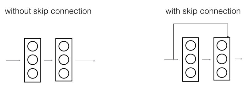
The image on the left shows the "main path" through the network. The image on the right adds a shortcut to the main path. By stacking these ResNet blocks on top of each other, you can form a very deep network.

ResNet blocks with the shortcut also make it very easy for one to learn an identity function. This means that you can stack on additional ResNet blocks with little risk of harming training set performance. There is also evidence that the ease of learning an identity function--even more than skip connections helping with vanishing gradients--accounts for ResNets' remarkable performance.

Two main blocks are used in a ResNet, depending mainly on whether the input/output dimensions are the same or different. We are going to implement both of them. Why do Skip Connections work?

• They mitigate the problem of vanishing gradient by allowing this alternate shortcut path for the gradient to flow through;
• They allow the model to learn an identity function which ensures that the higher layer will perform at least as good as the lower layer and not worse.

2.1 - The identity block:

To flesh out the different steps of what happens in a ResNet's identity block. The identity block is the standard block used in ResNets and corresponds to the case where the input activation (say a[l]) has the same dimension as the output activation (say a[l+2]). We'll actually implement a slightly more powerful version of this identity block, in which the skip connection "skips over" 3 hidden layers rather than 2 layers:

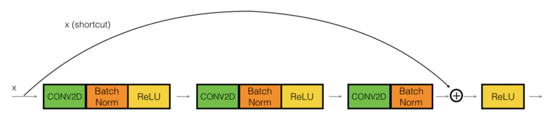
The upper path is the "shortcut path." The lower path is the "main path." In this diagram, we have also made explicit the CONV2D and ReLU steps in each layer. Here're the individual steps:

The first component of the main path:

• The first CONV2D has F1 filters of shape (1,1) and a stride of (1,1). Its padding is "valid" and its name should be conv_name_base + '2a'. Use 0 as the seed for the random initialization;
• The first BatchNorm is normalizing the channels axis. Its name should be bn_name_base + '2a';
• Then apply the ReLU activation function. This has no name and no hyperparameters.

The second component of the main path:

• The first CONV2D has F2 filters of shape (1,1) and a stride of (1,1). Its padding is "valid" and its name should be conv_name_base + '2b'. Use 0 as the seed for the random initialization;
• The first BatchNorm is normalizing the channels axis. Its name should be bn_name_base + '2b';
• Then apply the ReLU activation function. This has no name and no hyperparameters.

The third component of the main path:

• The first CONV2D has F3 filters of shape (1,1) and a stride of (1,1). Its padding is "valid" and its name should be conv_name_base + '2c'. Use 0 as the seed for the random initialization;
• The third BatchNorm is normalizing the channels axis. Its name should be bn_name_base + '2c'. Note that there is no ReLU activation function in this component.

Final step:

• The shortcut and the input are added together;
• Then apply the ReLU activation function. This has no name and no hyperparameters.

Arguments:

X - input tensor of shape (m, n_H_prev, n_W_prev, n_C_prev);
f - integer, specifying the shape of the middle CONV's window for the main path;
filters - python list of integers, defining the number of filters in the CONV layers of the main path;
stage - integer, used to name the layers, depending on their position in the network;
block - string/character, used to name the layers, depending on their position in the network.

Returns:

X - output of the identity block, tensor of shape (n_H, n_W, n_C)

def identity_block(X, f, filters, stage, block):
    # defining name basis
    conv_name_base = 'res' + str(stage) + block + '_branch'
    bn_name_base = 'bn' + str(stage) + block + '_branch'

    # Retrieve Filters
    F1, F2, F3 = filters

    # Save the input value. We'll need this later to add back to the main path. 
    X_shortcut = X

    # First component of main path
    X = Conv2D(filters = F1, kernel_size = (1, 1), strides = (1,1), padding = 'valid', name = conv_name_base + '2a', kernel_initializer = glorot_uniform(seed=0))(X)
    X = BatchNormalization(axis = 3, name = bn_name_base + '2a')(X)
    X = Activation('relu')(X)

    # Second component of main path
    X = Conv2D(filters = F2, kernel_size = (f, f), strides = (1,1), padding = 'same', name = conv_name_base + '2b', kernel_initializer = glorot_uniform(seed=0))(X)
    X = BatchNormalization(axis = 3, name = bn_name_base + '2b')(X)
    X = Activation('relu')(X)

    # Third component of main path
    X = Conv2D(filters = F3, kernel_size = (1, 1), strides = (1,1), padding = 'valid', name = conv_name_base + '2c', kernel_initializer = glorot_uniform(seed=0))(X)
    X = BatchNormalization(axis = 3, name = bn_name_base + '2c')(X)

    # Final step: Add shortcut value to main path, and pass it through a RELU activation
    X = Add()([X, X_shortcut])
    X = Activation('relu')(X)

    return X

tf.reset_default_graph()
with tf.Session() as test:
    A_prev = tf.placeholder("float", [3, 4, 4, 6])
    X = np.random.randn(3, 4, 4, 6)
    A = identity_block(A_prev, f = 2, filters = [2, 4, 6], stage = 1, block = 'a')
    test.run(tf.global_variables_initializer())
    out = test.run([A], feed_dict={A_prev: X, K.learning_phase(): 0})
    print("out = ", out[0][1][1][0])

Output:

out =  [1.2611859 2.0174022 2.8489313 2.459698  4.33884   2.1486042]

2.2 - The convolutional block:

The ResNet "convolutional block" is the other type of block:

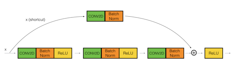
The CONV2D layer in the shortcut path is used to resize the input 𝑥 to a different dimension so that the dimensions match up in the final addition needed to add the shortcut value back to the main path. For example, to reduce the activation dimensions' height and width by a factor of 2, we can use a 1x1 convolution with a stride of 2. The CONV2D layer on the shortcut path does not use any non-linear activation function. Its main role is to apply a (learned) linear function that reduces the input dimension so that the dimensions match up for the later addition step.

The details of the convolutional block are as follows:

The first component of the main path:

• The first CONV2D has F1 filters of shape (1,1) and a stride of (1,1). Its padding is "valid" and its name should be conv_name_base + '2a'. Use 0 as the seed for the random initialization.
• The first BatchNorm is normalizing the channels axis. Its name should be bn_name_base + '2a'.
• Then apply the ReLU activation function. This has no name and no hyperparameters.

The second component of the main path:

• The first CONV2D has F₂ filters of shape (1,1) and a stride of (1,1). Its padding is "valid" and its name should be conv_name_base + '2b'. Use 0 as the seed for the random initialization;
• The first BatchNorm is normalizing the channels axis. Its name should be bn_name_base + '2b';
• Then apply the ReLU activation function. This has no name and no hyperparameters.

The third component of the main path:

• The first CONV2D has F₃ filters of shape (1,1) and a stride of (1,1). Its padding is "valid" and its name should be conv_name_base + '2c'. Use 0 as the seed for the random initialization;
• The third BatchNorm is normalizing the channels axis. Its name should be bn_name_base + '2c'. Note that there is no ReLU activation function in this component.

Shortcut path:

• The CONV2D has F₃ filters of shape (1,1) and a stride of (s,s). Its padding is "valid" and its name should be conv_name_base + '1';
• The BatchNorm is normalizing the channels axis. Its name should be bn_name_base + '1'.

Final step:

• The shortcut and the input are added together;
• Then apply the ReLU activation function. This has no name and no hyperparameters.

Arguments:

X - input tensor of shape (m, n_H_prev, n_W_prev, n_C_prev);
f - integer, specifying the shape of the middle CONV's window for the main path;
filters - python list of integers, defining the number of filters in the CONV layers of the main path;
stage - integer, used to name the layers, depending on their position in the network;
block - string/character, used to name the layers, depending on their position in the network;
s - Integer, specifying the stride to be used.

Returns:

X - output of the convolutional block, tensor of shape (n_H, n_W, n_C).

def convolutional_block(X, f, filters, stage, block, s = 2):
    # defining name basis
    conv_name_base = 'res' + str(stage) + block + '_branch'
    bn_name_base = 'bn' + str(stage) + block + '_branch'
    
    # Retrieve Filters
    F1, F2, F3 = filters
    
    # Save the input value
    X_shortcut = X


    ##### MAIN PATH #####
    # First component of main path 
    X = Conv2D(F1, (1, 1), strides = (s,s), name = conv_name_base + '2a', kernel_initializer = glorot_uniform(seed=0))(X)
    X = BatchNormalization(axis = 3, name = bn_name_base + '2a')(X)
    X = Activation('relu')(X)

    # Second component of main path
    X = Conv2D(filters=F2, kernel_size=(f, f), strides=(1, 1), padding='same', name=conv_name_base + '2b', kernel_initializer=glorot_uniform(seed=0))(X)
    X = BatchNormalization(axis=3, name=bn_name_base + '2b')(X)
    X = Activation('relu')(X)

    # Third component of main path
    X = Conv2D(filters=F3, kernel_size=(1, 1), strides=(1, 1), padding='valid', name=conv_name_base + '2c', kernel_initializer=glorot_uniform(seed=0))(X)
    X = BatchNormalization(axis=3, name=bn_name_base + '2c')(X)

    
    ##### SHORTCUT PATH ####
    X_shortcut = Conv2D(F3, (1, 1), strides = (s,s), name = conv_name_base + '1', kernel_initializer = glorot_uniform(seed=0))(X_shortcut)
    X_shortcut = BatchNormalization(axis = 3, name = bn_name_base + '1')(X_shortcut)

    # Final step: Add shortcut value to main path, and pass it through a RELU activation
    X = Add()([X, X_shortcut])
    X = Activation('relu')(X)
    
    return X

tf.reset_default_graph()
with tf.Session() as test:
    A_prev = tf.placeholder("float", [3, 4, 4, 6])
    X = np.random.randn(3, 4, 4, 6)
    A = convolutional_block(A_prev, f = 2, filters = [2, 4, 6], stage = 1, block = 'a')
    test.run(tf.global_variables_initializer())
    out = test.run([A], feed_dict={A_prev: X, K.learning_phase(): 0})
    print("out = ",out[0][1][1][0])

Output:

out =  [0.45051736, 0., 0.8701941,  0., 1.8204272, 0.]

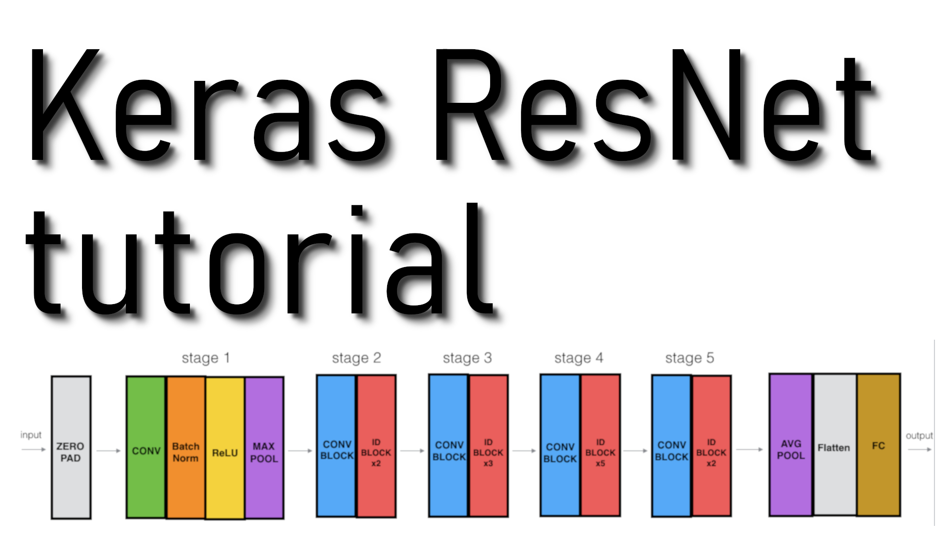
3 - Building our first ResNet model (50 layers):

We now have the necessary blocks to build a very deep ResNet. The following figure describes in detail the architecture of this neural network. "ID BLOCK" in the diagram stands for "Identity block," and "ID BLOCK x3" means you should stack 3 identity blocks together.

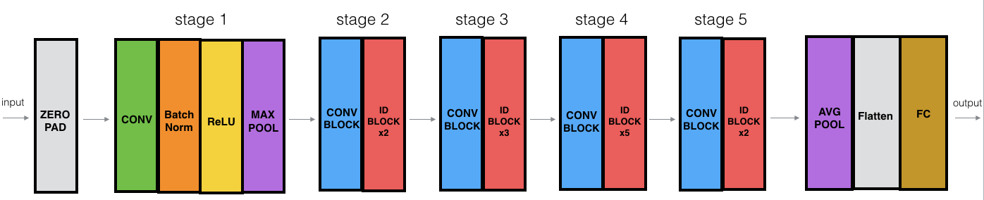
The details of this ResNet-50 model are:

• Zero-padding pads the input with a pad of (3,3);
• Stage 1:
• The 2D Convolution has 64 filters of shape (7,7) and uses a stride of (2,2). Its name is "conv1";
• BatchNorm is applied to the channels axis of the input;
• MaxPooling uses a (3,3) window and a (2,2) stride.
• Stage 2:
• The convolutional block uses three set of filters of size [64,64,256], "f" is 3, "s" is 1, and the block is "a";
• The 2 identity blocks use three sets of filters of size [64,64,256], "f" is 3, and the blocks are "b" and "c".
• Stage 3:
• The convolutional block uses three sets of filters of size [128,128,512], "f" is 3, "s" is 2, and the block is "a";
• The 3 identity blocks use three set of filters of size [128,128,512], "f" is 3 and the blocks are "b", "c" and "d".
• Stage 4:
• The convolutional block uses three sets of filters of size [256, 256, 1024], "f" is 3, "s" is 2, and the block is "a";
• The 5 identity blocks use three set of filters of size [256, 256, 1024], "f" is 3 and the blocks are "b", "c", "d", "e" and "f".
• Stage 5:
• The convolutional block uses three set of filters of size [512, 512, 2048], "f" is 3, "s" is 2, and the block is "a";
• The 2 identity blocks use three sets of filters of size [512, 512, 2048], "f" is 3, and the blocks are "b" and "c".
• The 2D Average Pooling uses a window of shape (2,2), and its name is "avg_pool";
• The flatten doesn't have any hyperparameters or names;
• The Fully Connected (Dense) layer reduces its input to the number of classes using a softmax activation. Its name should be 'fc' + str(classes).

So we will implement the ResNet with 50 layers described in the figure above into the following architecture:
CONV2D -> BATCHNORM -> RELU -> MAXPOOL -> CONVBLOCK -> IDBLOCK2 -> CONVBLOCK -> IDBLOCK3 -> CONVBLOCK -> IDBLOCK5 -> CONVBLOCK -> IDBLOCK2 -> AVGPOOL -> TOPLAYER.

Arguments:

input_shape - the shape of the images of the dataset;
classes - integer, number of classes.

Returns:

model - a Model() instance in Keras

def ResNet50(input_shape = (64, 64, 3), classes = 2):   
    # Define the input as a tensor with shape input_shape
    X_input = Input(input_shape)

    # Zero-Padding
    X = ZeroPadding2D((3, 3))(X_input)
    
    # Stage 1
    X = Conv2D(64, (7, 7), strides = (2, 2), name = 'conv1', kernel_initializer = glorot_uniform(seed=0))(X)
    X = BatchNormalization(axis = 3, name = 'bn_conv1')(X)
    X = Activation('relu')(X)
    X = MaxPooling2D((3, 3), strides=(2, 2))(X)

    # Stage 2
    X = convolutional_block(X, f = 3, filters = [64, 64, 256], stage = 2, block='a', s = 1)
    X = identity_block(X, 3, [64, 64, 256], stage=2, block='b')
    X = identity_block(X, 3, [64, 64, 256], stage=2, block='c')

    # Stage 3
    X = convolutional_block(X, f = 3, filters = [128, 128, 512], stage = 3, block='a', s = 2)
    X = identity_block(X, 3, [128, 128, 512], stage=3, block='b')
    X = identity_block(X, 3, [128, 128, 512], stage=3, block='c')
    X = identity_block(X, 3, [128, 128, 512], stage=3, block='d')

    # Stage 4
    X = convolutional_block(X, f = 3, filters = [256, 256, 1024], stage = 4, block='a', s = 2)
    X = identity_block(X, 3, [256, 256, 1024], stage=4, block='b')
    X = identity_block(X, 3, [256, 256, 1024], stage=4, block='c')
    X = identity_block(X, 3, [256, 256, 1024], stage=4, block='d')
    X = identity_block(X, 3, [256, 256, 1024], stage=4, block='e')
    X = identity_block(X, 3, [256, 256, 1024], stage=4, block='f')

    # Stage 5
    X = convolutional_block(X, f = 3, filters = [512, 512, 2048], stage = 5, block='a', s = 2)
    X = identity_block(X, 3, [512, 512, 2048], stage=5, block='b')
    X = identity_block(X, 3, [512, 512, 2048], stage=5, block='c')

    # AVGPOOL.
    X = AveragePooling2D((2, 2), name='avg_pool')(X)

    # output layer
    X = Flatten()(X)
    X = Dense(classes, activation='softmax', name='fc' + str(classes), kernel_initializer = glorot_uniform(seed=0))(X)
    
    # Create model
    model = Model(inputs = X_input, outputs = X, name='ResNet50')

    return model

Run the following code to build the model's graph. If your implementation is not correct, you will know it by checking your accuracy when running model.fit(...) below:

model = ResNet50(input_shape = (ROWS, COLS, CHANNELS), classes = CLASSES)

Now we need to configure the learning process by compiling the model:

model.compile(optimizer='adam', loss='categorical_crossentropy', metrics=['accuracy'])

The model is now ready to be trained. Run the following cell to train your model on 100 epochs with a batch size of 64:

model.fit(X_train, Y_train, epochs = 100, batch_size = 64)

6002/6002 [=================] - 12s 2ms/step - loss: 0.0403 - acc: 0.9900
Epoch 99/100
6002/6002 [=================] - 13s 2ms/step - loss: 0.0148 - acc: 0.9947
Epoch 100/100
6002/6002 [=================] - 14s 2ms/step - loss: 0.0289 - acc: 0.9902

Let's see how this model (trained on 100 epochs) performs on the test set.

preds = model.evaluate(X_test, Y_test)
print ("Loss = " + str(preds[0]))
print ("Test Accuracy = " + str(preds[1]))

1000/1000 [=================] - 2s 2ms/step
Loss = 1.3275088095664977
Test Accuracy = 0.724

We can also print a summary of our model by running the following code:

model.summary()

For future use, we can save our model to a file:

model.save('ResNet50.h5')

Finally, we can run the code below to visualize our ResNet50:

plot_model(model, to_file='model.png')
SVG(model_to_dot(model).create(prog='dot', format='svg'))

What you should remember:

• Very deep "plain" networks don't work in practice because they are hard to train due to vanishing gradients;
• The skip-connections help to address the Vanishing Gradient problem. They also make it easy for a ResNet block to learn an identity function;
• There are two main types of blocks: The identity block and the convolutional block;
• Very deep Residual Networks are built by stacking these blocks together.