Build our first Convolutional Neural Network

Welcome to 4th tutorial part! In this part, we will:

• Implement helper functions that we will use when implementing a TensorFlow model;
• Implement a fully functioning ConvNet using TensorFlow.

After this tutorial, we will be able to:

• Build and train a ConvNet in TensorFlow for a classification problem.

TensorFlow model:

In the previous tutorial, we built Deep Neural Networks using TensorFlow. Today's most practical applications of deep learning are built using programming frameworks, which have many built-in functions you can call. As usual, we will start by loading in the packages:

import os
os.environ['CUDA_VISIBLE_DEVICES'] = '0'
import cv2
import numpy as np
import matplotlib.pyplot as plt
import math
import tensorflow as tf

ROWS = 64
COLS = 64
CHANNELS = 3
CLASSES = 2

def read_image(file_path):
    img = cv2.imread(file_path, cv2.IMREAD_COLOR)
    return cv2.resize(img, (ROWS, COLS), interpolation=cv2.INTER_CUBIC)

def prepare_data(images):
    m = len(images)
    X = np.zeros((m, ROWS, COLS, CHANNELS), dtype=np.uint8)
    y = np.zeros((1, m), dtype=np.uint8)
    for i, image_file in enumerate(images):
        X[i,:] = read_image(image_file)
        if 'dog' in image_file.lower():
            y[0, i] = 1
        elif 'cat' in image_file.lower():
            y[0, i] = 0
    return X, y

def convert_to_one_hot(Y, C):
    Y = np.eye(C)[Y.reshape(-1)].T
    return Y

Run the next cell to load the "Cats vs. Dogs" data-set we are going to use:

TRAIN_DIR = 'Train_data/'
TEST_DIR = 'Test_data/'

train_images = [TRAIN_DIR+i for i in os.listdir(TRAIN_DIR)]
test_images =  [TEST_DIR+i for i in os.listdir(TEST_DIR)]

train_set_x, train_set_y = prepare_data(train_images)
test_set_x, test_set_y = prepare_data(test_images)

X_train = train_set_x/255
X_test = test_set_x/255

Y_train = convert_to_one_hot(train_set_y, CLASSES).T
Y_test = convert_to_one_hot(test_set_y, CLASSES).T

In the previous tutorial, we had built a fully connected Deep Network for this dataset. But since this is an image dataset, it is more natural to apply a ConvNet to it. To get started, let's examine the shapes of our data:

print ("number of training examples =", X_train.shape[0])
print ("number of test examples =", X_test.shape[0])
print ("X_train shape:", X_train.shape)
print ("Y_train shape:", Y_train.shape)
print ("X_test shape:", X_test.shape)
print ("Y_test shape:", Y_test.shape)

Output:

number of training examples = 6002
number of test examples = 1000
X_train shape: (6002, 64, 64, 3)
Y_train shape: (6002, 2)
X_test shape: (1000, 64, 64, 3)
Y_test shape: (1000, 2)

1 - Create placeholders:

TensorFlow requires that we create placeholders for the input data fed into the model when running the session. To do so, we could use "None" as the batch size. We will implement the function below to create placeholders for the input image X and the output Y. We should not define the number of training examples for the moment. It will give us the flexibility to choose it later.

Arguments:

n_H0 - scalar, the height of an input image;
n_W0 - scalar, the width of an input image;
n_C0 - scalar, number of channels of the input;
n_y - scalar, number of classes.

Returns:

X - placeholder for the data input, of shape [None, n_H0, n_W0, n_C0] and data type "float";
Y - placeholder for the input labels, shape [None, n_y], and data type "float".

def create_placeholders(n_H0, n_W0, n_C0, n_y):

    X = tf.placeholder(tf.float32, shape=(None, n_H0, n_W0, n_C0), name="X")
    Y = tf.placeholder(tf.float32, shape=(None, n_y), name="Y")
    
    return X, Y

X, Y = create_placeholders(ROWS, COLS, CHANNELS, CLASSES)
print ("X = ", X)
print ("Y = ", Y)

Output:

X =  Tensor("X_1:0", shape=(?, 64, 64, 3), dtype=float32)
Y =  Tensor("Y_1:0", shape=(?, 2), dtype=float32)

2 - Initialize parameters:

We will initialize weights/filters W1 and W2 using tf.contrib.layers.xavier_initializer(). We don't need to worry about bias variables as we will soon see that TensorFlow functions take care of the bias. Note also that we will only initialize the weights/filters for the conv2d functions. TensorFlow initializes the layers for the fully connected part automatically. We will talk more about that later.

The dimensions for each group of filters will be: [weight, height, channels, filters]

def initialize_parameters():
    
    W1 = tf.get_variable("W1", [4, 4, 3, 32], initializer = tf.contrib.layers.xavier_initializer())
    W2 = tf.get_variable("W2", [2, 2, 32, 32], initializer = tf.contrib.layers.xavier_initializer())

    parameters = {"W1": W1,
                  "W2": W2}
   
    return parameters

tf.reset_default_graph()
with tf.Session() as sess_test:
    parameters = initialize_parameters()
    init = tf.global_variables_initializer()
    sess_test.run(init)
    print("W1 = ", parameters["W1"].eval()[1,1,1])
    print("W2 = ", parameters["W2"].eval()[1,1,1])

Output:

W1 =  [-0.06732719 -0.04869158 -0.09797626  0.08584268  0.02240836  0.08350148
 -0.08144311  0.03549462  0.09043885 -0.00742315  0.07257762 -0.0955046
  0.06858646 -0.01282825 -0.04284175  0.04028637 -0.06008491 -0.07174417
 -0.02601603  0.06803527 -0.00658079 -0.06387079 -0.06514584  0.08079699
  0.0451208   0.09093665  0.02660077 -0.04926057 -0.01445787  0.01430324
 -0.0094941  -0.00567473]
W2 =  [-0.10164022  0.0088262   0.12092815  0.03691474  0.03909318 -0.11921392
 -0.11299625  0.13281281 -0.00964643  0.07956326  0.10702415 -0.02628222
  0.07636186  0.11758269 -0.07492408 -0.10864092 -0.03752776 -0.15154287
 -0.03635778 -0.07357109 -0.14489271 -0.09165138  0.03596993  0.09336357
  0.11486803  0.12517045 -0.1207674  -0.02368325 -0.04226575  0.06590688
 -0.03436987 -0.11981277]

3 - Forward propagation:

In TensorFlow, there are built-in functions that carry out the convolution steps for us.

• tf.nn.conv2d(X,W1, strides = [1,s,s,1], padding = 'SAME'): given an input X and a group of filters W1, this function convolves W1's filters on X. The third input ([1, f, f, 1]) represents the strides for each dimension of the input (m, n_H_prev, n_W_prev, n_C_prev).
• tf.nn.max_pool(A, ksize = [1,f,f,1], strides = [1,s,s,1], padding = 'SAME'): given an input A, this function uses a window of size (f, f) and strides of size (s, s) to carry out max-pooling over each window.
• tf.nn.relu(Z1): computes the elementwise ReLU of Z1 (which can be any shape).
• tf.contrib.layers.flatten(P): given an input P, this function flattens each example into a 1D vector while maintaining the batch size. It returns a flattened tensor with shape [batch_size, k].
• tf.contrib.layers.fully_connected(F, num_outputs): given a flattened input F, it returns the output computed using a fully connected layer.

In the last function above (tf.contrib.layers.fully_connected), the fully connected layer automatically initializes weights in the graph and keeps on training them as we train the model. We don't need to initialize those weights when initializing the parameters.

So we will implement the forward_propagation function below to build the following model: CONV2D -> RELU -> MAXPOOL -> CONV2D -> RELU -> MAXPOOL -> FLATTEN -> FULLYCONNECTED.

In detail, we will use the following parameters for all the steps: - Conv2D: stride 1, padding is "SAME":
- ReLU;
- Max pool: Use an 8 by 8 filter size and an 8 by 8 stride, padding is "SAME";
- Conv2D: stride 1, padding is "SAME";
- ReLU;
- Max pool: Use a 4 by 4 filter size and a 4 by 4 stride, padding is "SAME";
- Flatten the previous output.;
- FULLY CONNECTED (FC) layer: We'll apply a fully connected layer without a non-linear activation function. We will not call the softmax here. This will result in 2 neurons in the output layer, which get passed to a softmax layer. In TensorFlow, the softmax and cost function are lumped together into a single function, which you'll call in a different function when computing the cost.

Arguments:

X - input dataset placeholder, of shape (input size, number of examples);
parameters - python dictionary containing our parameters "W1", "W2".

Returns:

Z3 - the output of the last LINEAR unit.

def forward_propagation(X, parameters):
    # Retrieving the parameters from the dictionary "parameters" 
    W1 = parameters['W1']
    W2 = parameters['W2']
    
    # CONV2D: stride of 1, padding 'SAME'
    Z1 = tf.nn.conv2d(X,W1, strides = [1,1,1,1], padding = 'SAME')
    print("Z1 shape", Z1.shape)
    
    # RELU
    A1 = tf.nn.relu(Z1)
    print("A1 shape", A1.shape)
    
    # MAXPOOL: window 8x8, sride 8, padding 'SAME'
    P1 = tf.nn.max_pool(A1, ksize = [1,8,8,1], strides = [1,8,8,1], padding = 'SAME')
    print("P1 shape", P1.shape)
    
    # CONV2D: filters W2, stride 1, padding 'SAME'
    Z2 = tf.nn.conv2d(P1,W2, strides = [1,1,1,1], padding = 'SAME')
    print("Z2 shape", Z2.shape)
    
    # RELU
    A2 = tf.nn.relu(Z2)
    print("A2 shape", A2.shape)
    
    # MAXPOOL: window 4x4, stride 4, padding 'SAME'
    P2 = tf.nn.max_pool(A2, ksize = [1,4,4,1], strides = [1,4,4,1], padding = 'SAME')
    print("P2 shape", P2.shape)
    
    # FLATTEN
    P2 = tf.contrib.layers.flatten(P2)
    print("P2 FLATTEN shape", P2.shape)
    
    # FULLY-CONNECTED without non-linear activation function (not call softmax).
    # 2 neurons in output layer. Hint: one of the arguments should be "activation_fn=None" 
    Z3 = tf.contrib.layers.fully_connected(P2, CLASSES, activation_fn=None)
    print("Z3 shape", Z3.shape)

    return Z3

tf.reset_default_graph()
with tf.Session() as sess:
    X, Y = create_placeholders(ROWS, COLS, CHANNELS, CLASSES)
    parameters = initialize_parameters()
    Z3 = forward_propagation(X, parameters)
    init = tf.global_variables_initializer()
    sess.run(init)
    a = sess.run(Z3, {X: np.random.randn(2,64,64,3), Y: np.random.randn(2,CLASSES)})
    print("Z3 =", a)
    print("Z3 shape =", a.shape)

Output:

Z1 shape (?, 64, 64, 32)
A1 shape (?, 64, 64, 32)
P1 shape (?, 8, 8, 32)
Z2 shape (?, 8, 8, 32)
A2 shape (?, 8, 8, 32)
P2 shape (?, 2, 2, 32)
P2 FLATTEN shape (?, 128)
Z3 shape (?, 2)
Z3 = [[-1.3436915   0.34887427]
 [-1.5181915   0.01192094]]
Z3 shape = (2, 2)

4 - Compute cost:

In TensorFlow, there are built-in functions that carry out the convolution steps for us.

• tf.nn.softmax_cross_entropy_with_logits(logits = Z3, labels = Y): computes the softmax entropy loss. This function both computes the softmax activation function as well as the resulting loss;
• tf.reduce_mean: computes the mean of elements across dimensions of a tensor. Use this to sum the losses over all the examples to get the overall cost.

Arguments:

Z3 - output of the forward propagation (output of the last LINEAR unit), of shape (CLASSES, number of examples);
Y - "true" labels vector placeholder, the same shape as Z3.

Returns:

cost - Tensor of the cost function

def compute_cost(Z3, Y):

    cost = tf.reduce_mean(tf.nn.softmax_cross_entropy_with_logits(logits = Z3, labels = Y))
    
    return cost

tf.reset_default_graph()
with tf.Session() as sess:
    X, Y = create_placeholders(ROWS, COLS, CHANNELS, CLASSES)
    parameters = initialize_parameters()
    Z3 = forward_propagation(X, parameters)
    cost = compute_cost(Z3, Y)
    init = tf.global_variables_initializer()
    sess.run(init)
    a = sess.run(cost, {X: np.random.randn(4,64,64,3), Y: np.random.randn(4,CLASSES)})
    print("cost = ", a)

Output:

Z1 shape (?, 64, 64, 32)
A1 shape (?, 64, 64, 32)
P1 shape (?, 8, 8, 32)
Z2 shape (?, 8, 8, 32)
A2 shape (?, 8, 8, 32)
P2 shape (?, 2, 2, 32)
P2 FLATTEN shape (?, 128)
Z3 shape (?, 2)
cost =  1.4327825

5 - Mini-Batch Gradient descent:

I copied the mini-batches function from my last Deep Network TensorFlow tutorial and adapted it to a new data-set shape:

Arguments:

X - input data, of shape (input size, number of examples) (m, Hi, Wi, Ci);
Y - true "label" vector (containing 0 if cat, 1 if dog), of shape (1, number of examples) (m, n_y);
mini_batch_size - the size of the mini-batches, integer.

Returns:

mini_batches - list of synchronous (mini_batch_X, mini_batch_Y).

def random_mini_batches(X, Y, mini_batch_size = 64):
    # number of training examples
    m = X.shape[0]                  
    mini_batches = []
    
    # Step 1: Shuffle (X, Y)
    permutation = list(np.random.permutation(m))
    shuffled_X = X[permutation,:,:,:]
    shuffled_Y = Y[permutation,:]

    # Step 2: Partition (shuffled_X, shuffled_Y). Minus the end case.
    num_complete_minibatches = math.floor(m/mini_batch_size) # number of mini batches of size mini_batch_size in your partitionning
    for k in range(0, num_complete_minibatches):
        mini_batch_X = shuffled_X[k * mini_batch_size : k * mini_batch_size + mini_batch_size,:,:,:]
        mini_batch_Y = shuffled_Y[k * mini_batch_size : k * mini_batch_size + mini_batch_size,:]
        mini_batch = (mini_batch_X, mini_batch_Y)
        mini_batches.append(mini_batch)
    
    # Handling the end case (last mini-batch < mini_batch_size)
    if m % mini_batch_size != 0:
        mini_batch_X = shuffled_X[num_complete_minibatches * mini_batch_size : m,:,:,:]
        mini_batch_Y = shuffled_Y[num_complete_minibatches * mini_batch_size : m,:]
        mini_batch = (mini_batch_X, mini_batch_Y)
        mini_batches.append(mini_batch)
    
    return mini_batches

6 - Model:

Finally, we will merge the helper functions we implemented above to build a model. We will train it on my Cats and Dogs data-set.

The model below should:

• create placeholders;
• initialize parameters;
• forward propagate;
• compute the cost;
• create an optimizer.

Finally, we will create a session and run a for loop for num_epochs, get the mini-batches, and then for each mini-batch, we will optimize the function. So we'll implement a three-layer ConvNet in Tensorflow: CONV2D -> RELU -> MAXPOOL -> CONV2D -> RELU -> MAXPOOL -> FLATTEN -> FULLY CONNECTED.

Arguments:

X_train - training set, of shape (None, ROWS, COLS, CHANNELS);
Y_train - test set, of shape (None, n_y = CLASSES);
X_test - training set, of shape (None, ROWS, COLS, CHANNELS);
Y_test - test set, of shape (None, n_y = CLASSES);
learning_rate - learning rate of the optimization;
num_epochs - number of epochs of the optimization loop;
minibatch_size - the size of a minibatch;
print_cost - True to print the cost every 100 epochs.

Returns:

train_accuracy - real number, accuracy on the train set (X_train);
test_accuracy - real number, testing accuracy on the test set (X_test);
parameters - parameters learned by the model. They can then be used to predict.

tf.reset_default_graph()
def model(X_train, Y_train, X_test, Y_test, learning_rate = 0.009,
          num_epochs = 200, minibatch_size = 64, print_cost = True):

    (m, n_H0, n_W0, n_C0) = X_train.shape             
    n_y = Y_train.shape[1] 
    
    # To keep track of the cost
    costs = []                                        
    
    # Createing Placeholders of the correct shape
    X, Y = create_placeholders(n_H0, n_W0, n_C0, n_y)

    # Initializing parameters
    parameters = initialize_parameters()
    
    # Forward propagation: Building the forward propagation in the tensorflow graph
    Z3 = forward_propagation(X, parameters)
    
    # Cost function: Adding cost function to tensorflow graph
    cost = compute_cost(Z3, Y)
    
    # Backpropagation: Defining the tensorflow optimizer. Using an AdamOptimizer that minimizes the cost.
    optimizer = tf.train.AdamOptimizer(learning_rate = learning_rate).minimize(cost)
    
    # Initializing all the variables globally
    init = tf.global_variables_initializer()
     
    # Starting the session to compute the tensorflow graph
    with tf.Session() as sess:
        
        # Runing the initialization
        sess.run(init)
        
        # Doing the training loop
        for epoch in range(num_epochs):

            minibatch_cost = 0.
            # number of minibatches of size minibatch_size in the train set
            num_minibatches = int(m / minibatch_size)
            minibatches = random_mini_batches(X_train, Y_train, minibatch_size)

            for minibatch in minibatches:

                # Select a minibatch
                (minibatch_X, minibatch_Y) = minibatch
                # IMPORTANT: The line that runs the graph on a minibatch.
                # Run the session to execute the optimizer and the cost, the feedict should contain a minibatch for (X,Y).
                _ , temp_cost = sess.run([optimizer, cost], feed_dict={X: minibatch_X, Y: minibatch_Y})
                
                minibatch_cost += temp_cost / num_minibatches
                

            # Print the cost every epoch
            if print_cost == True and epoch % 5 == 0:
                print ("Cost after epoch %i: %f" % (epoch, minibatch_cost))
            if print_cost == True and epoch % 1 == 0:
                costs.append(minibatch_cost)
        
        
        # plot the cost
        plt.plot(np.squeeze(costs))
        plt.ylabel('cost')
        plt.xlabel('iterations (per tens)')
        plt.title("Learning rate =" + str(learning_rate))
        plt.show()
        
        # lets save the parameters in a variable
        parameters = sess.run(parameters)
        print ("Parameters have been trained!")     
        
        # Calculate the correct predictions
        predict_op = tf.argmax(Z3, 1)
        correct_prediction = tf.equal(predict_op, tf.argmax(Y, 1))
        
        # Calculate accuracy on the test set
        accuracy = tf.reduce_mean(tf.cast(correct_prediction, "float"))
        train_accuracy = accuracy.eval({X: X_train, Y: Y_train})
        test_accuracy = accuracy.eval({X: X_test, Y: Y_test})
        print("Train Accuracy:", train_accuracy)
        print("Test Accuracy:", test_accuracy)
        
        # Saving our trained model
        saver = tf.train.Saver()
        tf.add_to_collection('predict_op', predict_op)
        saver.save(sess, './my-CNN-model')        
                
        return train_accuracy, test_accuracy, parameters

Run the following cell to train your model for 200 epochs:

_, _, parameters = model(X_train, Y_train, X_test, Y_test)

Output:

Z1 shape (?, 64, 64, 32)
A1 shape (?, 64, 64, 32)
P1 shape (?, 8, 8, 32)
Z2 shape (?, 8, 8, 32)
A2 shape (?, 8, 8, 32)
P2 shape (?, 2, 2, 32)
P2 FLATTEN shape (?, 128)
Z3 shape (?, 2)
Cost after epoch 0: 0.701049
Cost after epoch 5: 0.580966
Cost after epoch 10: 0.525494
Cost after epoch 15: 0.509302
...
...
Cost after epoch 195: 0.230628

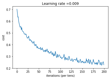
Parameters have been trained!
Train Accuracy: 0.92952347
Test Accuracy: 0.703

7 - Test with your own image:

When we save the variables, it creates a .meta file. This file contains the graph structure. Therefore, we can import the meta graph using tf.train.import_meta_graph() and restore the values of the graph. Let's import the graph and see all tensors in the graph:

# delete the current graph
tf.reset_default_graph()

# import the graph from the file
imported_graph = tf.train.import_meta_graph('my-CNN-model.meta')

# list all the tensors in the graph
for tensor in tf.get_default_graph().get_operations():
    print (tensor.name)

We can now take a picture of our cat or dog and see the output of our model. To do that:

#test_image = "cat.jpg"
test_image = "dog.jpg"
my_image = read_image(test_image).reshape(1, ROWS, COLS, CHANNELS)
X = my_image / 255.
#print(X.shape)

checkpoint_path = 'my-CNN-model'
tf.reset_default_graph()

with tf.Session() as sess:

    ## Load the entire model previuosly saved in a checkpoint
    print("Load the model from path", checkpoint_path)
    the_Saver = tf.train.import_meta_graph(checkpoint_path + '.meta')
    the_Saver.restore(sess, checkpoint_path)

    ## Identify the predictor of the Tensorflow graph
    predict_op = tf.get_collection('predict_op')[0]

    ## Identify the restored Tensorflow graph
    dataFlowGraph = tf.get_default_graph()

    ## Identify the input placeholder to feed the images into as defined in the model 
    x = dataFlowGraph.get_tensor_by_name("X:0")

    ## Predict the image category
    prediction = sess.run(predict_op, feed_dict = {x: X})

    print("\nThe predicted image class is:", np.squeeze(prediction))

Conclusion: