Building our first neural network in TensorFlow:
In this tutorial part, we will build a deep neural network using TensorFlow. Remember that there are two parts to implement a TensorFlow model:
- Create the computation graph
- Run the graph
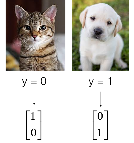
In this part, we'll use the same Cats vs. Dogs data-set we used in our previous tutorials. But in this tutorial, instead of using sigmoid, we'll use the softmax function, so if you want, you can add more classes to recognize. Also, because we'll use softmax, we need to change the shape of our labels, so I made the convert_to_one_hot function. You know what it does if you watched my previous tutorial. Adding to this, our used data shape will be a little different than we used before; everything is in the following lines:
As usual, we flatten the image dataset, then normalize it by dividing it by 255. On top of that, we will convert each label to a one-hot vector:
print ("number of training examples =", X_train.shape[1])
print ("number of test examples =", X_test.shape[1])
print ("X_train shape:", X_train.shape)
print ("Y_train shape:", Y_train.shape)
print ("X_test shape:", X_test.shape)
print ("Y_test shape:", Y_test.shape)
Output:
number of training examples = 6002
number of test examples = 1000
X_train shape: (12288, 6002)
Y_train shape: (2, 6002)
X_test shape: (12288, 1000)
Y_test shape: (2, 1000)
Note that 12288 comes from 64×64×3. Each image is square, 64 by 64 pixels, and 3 is for the RGB colors. Please make sure all these shapes make sense to you before continuing.
Our goal is to build an algorithm capable of recognizing a cat and dog with high accuracy. To do so, we will build a TensorFlow model that is almost the same as one we have previously built in NumPy for cat recognition (but now using a softmax output). It is a great occasion to compare your NumPy implementation to the TensorFlow one. You'll see that the training of the model on TensorFlow is significantly faster.
The model will be LINEAR -> RELU -> LINEAR -> RELU -> LINEAR -> SOFTMAX. The SIGMOID output layer has been converted to a SOFTMAX. A SOFTMAX layer generalizes SIGMOID to when there are more than two classes.
1 - Create placeholders:
Our first task is to create placeholders for X and Y`. This will allow us later ta pass our training data in when we run our session. Below is function to create the placeholders in TensorFlow:
Arguments:
n_x - scalar, size of an image vector (num_px * num_px = ROWS * COLS * CHANNELS = 12288);
n_y - scalar, number of classes (from 0 to 1, so -> 2).
Returns:
X - placeholder for the data input, of shape [n_x, None] and data type "float";
Y - placeholder for the input labels, shape [n_y, None], and data type "float".
Tips:
We will use None because it lets us be flexible on the number of examples for the placeholders.
In fact, the number of examples during test/train is different.
def create_placeholders(n_x, n_y):

    X = tf.placeholder(tf.float32, shape=(n_x, None), name = 'X')
    Y = tf.placeholder(tf.float32, shape=(n_y, None), name = 'Y')

    return X, Y

X, Y = create_placeholders(X_train.shape[0], CLASSES)
print ("X = " + str(X))
print ("Y = " + str(Y))
Output:
X = Tensor("X_1:0", shape=(12288, ?), dtype=float32)
Y = Tensor("Y_1:0", shape=(2, ?), dtype=float32)
2 - Initializing the parameters:
Our second task is to initialize the parameters in TensorFlow. We are going to use Xavier Initialization for weights and Zero Initialization for biases.
Arguments:
INPUT, h1, h2, OUTPUT - size of model layers
Returns:
parameters - a dictionary of tensors containing W1, b1, W2, b2, W3, b3
def initialize_parameters(INPUT, h1, h2, OUTPUT):
    W1 = tf.get_variable("W1", [h1, INPUT], initializer = tf.contrib.layers.xavier_initializer())
    b1 = tf.get_variable("b1", [h1, 1], initializer = tf.zeros_initializer())
    W2 = tf.get_variable("W2", [h2, h1], initializer = tf.contrib.layers.xavier_initializer())
    b2 = tf.get_variable("b2", [h2, 1], initializer = tf.zeros_initializer())
    W3 = tf.get_variable("W3", [OUTPUT, h2], initializer = tf.contrib.layers.xavier_initializer())
    b3 = tf.get_variable("b3", [OUTPUT, 1], initializer = tf.zeros_initializer())


    parameters = {"W1": W1,
                  "b1": b1,
                  "W2": W2,
                  "b2": b2,
                  "W3": W3,
                  "b3": b3}

    return parameters

tf.reset_default_graph()
with tf.Session() as sess:
    parameters = initialize_parameters(X_train.shape[0], 25, 12, CLASSES)
    print("W1 = ", parameters["W1"])
    print("b1 = ", parameters["b1"])
    print("W2 = ", parameters["W2"])
    print("b2 = ", parameters["b2"])
    print("W3 = ", parameters["W3"])
    print("b3 = ", parameters["b3"])
Output:
W1 = <tf.Variable 'W1:0' shape=(25, 12288) dtype=float32_ref>
b1 = <tf.Variable 'b1:0' shape=(25, 1) dtype=float32_ref>
W2 = <tf.Variable 'W2:0' shape=(12, 25) dtype=float32_ref>
b2 = <tf.Variable 'b2:0' shape=(12, 1) dtype=float32_ref>
W3 = <tf.Variable 'W3:0' shape=(2, 12) dtype=float32_ref>
b3 = <tf.Variable 'b3:0' shape=(2, 1) dtype=float32_ref>
3 - Forward propagation in TensorFlow:
We will now implement the forward propagation module in TensorFlow. The function will take in a dictionary of parameters, and it will complete the forward pass. The functions we will be using are:
tf.add(..., ...)to do an addition;tf.matmul(..., ...)to do a matrix multiplication;tf.nn.relu(...)to apply the ReLU activation.
Note: I commented on the numpy equivalents so that you can compare the TensorFlow implementation to numpy. It is important to note that the forward propagation stops at z3. In TensorFlow, the last linear layer output is given as input to the function computing the loss. Therefore, you don't need a3!
Arguments:
X - input dataset placeholder, of shape (input size, number of examples);
parameters - python dictionary containing our parameters "W1", "b1", "W2", "b2", "W3", "b3" the shapes are given in initialize_parameters.
Returns:
Z3 - the output of the last LINEAR unit.
def forward_propagation(X, parameters):
    # Retrieving parameters from the dictionary "parameters"
    W1 = parameters['W1']
    b1 = parameters['b1']
    W2 = parameters['W2']
    b2 = parameters['b2']
    W3 = parameters['W3']
    b3 = parameters['b3']

                                      # Numpy Equivalents:
    Z1 = tf.add(tf.matmul(W1,X),b1)   # Z1 = np.dot(W1, X) + b1
    A1 = tf.nn.relu(Z1)               # A1 = relu(Z1)
    Z2 = tf.add(tf.matmul(W2,A1),b2)  # Z2 = np.dot(W2, a1) + b2
    A2 = tf.nn.relu(Z2)               # A2 = relu(Z2)
    Z3 = tf.add(tf.matmul(W3,A2),b3)  # Z3 = np.dot(W3,Z2) + b3

    return Z3

tf.reset_default_graph()

with tf.Session() as sess:
    X, Y = create_placeholders(X_train.shape[0], CLASSES)
    parameters = initialize_parameters(X_train.shape[0], 25, 12, CLASSES)
    Z3 = forward_propagation(X, parameters)
    print("Z3 =", Z3)
Output:
Z3 = Tensor("Add_2:0", shape=(2, ?), dtype=float32)You may have noticed that the forward propagation doesn't output any cache. Soon you will understand why when we get to backpropagation.
4 - Compute cost:
As seen before, it is straightforward to compute the cost using:
tf.reduce_mean(tf.nn.softmax_cross_entropy_with_logits(logits = ..., labels = ...))
Note:
- It is important to know that the "logits" and "labels" inputs of
tf.nn.softmax_cross_entropy_with_logitsare expected to be of shape (number of examples, num_classes), so I have transposed Z3 and Y for you; - Besides,
tf.reduce_meanbasically does the summation over the examples.
Arguments:
Z3 - output of forwarding propagation (output of the last LINEAR unit), of shape (CLASSES, number of examples);
Y - "true" labels vector placeholder, the same shape as Z3.
Returns:
cost - Tensor of the cost function.
def compute_cost(Z3, Y):
    # fit the tensorflow requirement for tf.nn.softmax_cross_entropy_with_logits(...,...)
    logits = tf.transpose(Z3)
    labels = tf.transpose(Y)

    cost = tf.reduce_mean(tf.nn.softmax_cross_entropy_with_logits(logits = logits, labels = labels))

    return cost

tf.reset_default_graph()

with tf.Session() as sess:
    X, Y = create_placeholders(X_train.shape[0], CLASSES)
    parameters = initialize_parameters(X_train.shape[0], 25, 12, CLASSES)
    Z3 = forward_propagation(X, parameters)
    cost = compute_cost(Z3, Y)
    print("cost =",cost)
Output:
cost = Tensor("Mean:0", shape=(), dtype=float32)
5 - Mini-Batch Gradient descent:
Let's build mini-batches from the training set (X, Y) in two steps:
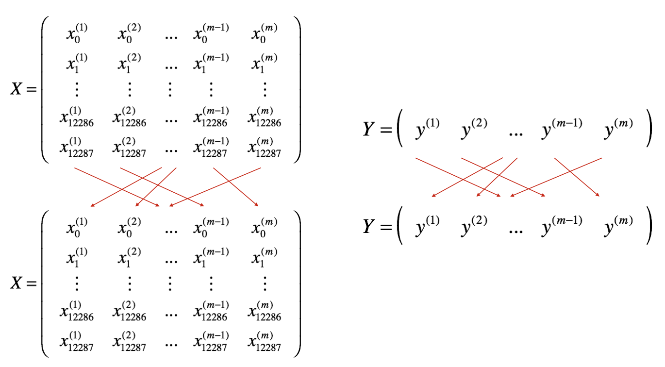
Shuffle: We'll create a shuffled version of the training set (X, Y), as shown below. Each column of X and Y represents a training example. Note that the random shuffling is done synchronously between X and Y. Such that after the shuffling, the ith column of X is the example corresponding to the ith label in Y. The shuffling step ensures that examples will be split randomly into different mini-batches.
ini_batch_size. The last mini-batch might be smaller, but you don't need to worry about this. When the final mini-batch is smaller than the full mini_batch_size, it will look like this: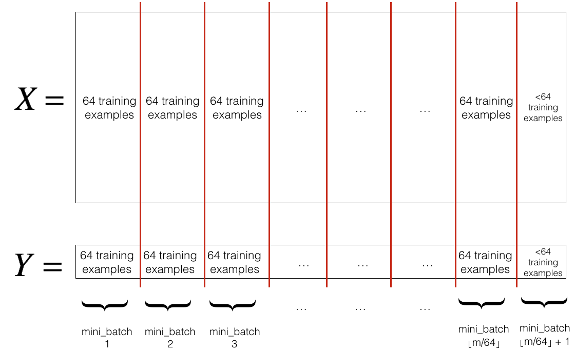
mini_batch_size=64 let [s] represents s rounded down to the nearest integer (this is math.floor(s) function in Python). If the total number of examples is not a multiple of mini_batch_size=64 then there will be [m / mmini_batch_size] mini-batches with a full 64 examples, and the number of examples in the final mini-batch will be (m−mini_batch_size*[m / mmini_batch_size]).Y - true "label" vector (containing 0 if cat, 1 if non-cat), of shape (1, number of examples);
mini_batch_size - the size of the mini-batches, integer.
def random_mini_batches(X, Y, mini_batch_size = 64):
    # number of training examples
    m = X.shape[1]
    mini_batches = []

    # Step 1: Shuffle (X, Y)
    permutation = list(np.random.permutation(m))
    shuffled_X = X[:, permutation]
    shuffled_Y = Y[:, permutation].reshape((Y.shape[0],m))

    # Step 2: Partition (shuffled_X, shuffled_Y). Minus the end case.
    # number of mini batches of size mini_batch_size in your partitionning
    num_complete_minibatches = math.floor(m/mini_batch_size)
    for k in range(0, num_complete_minibatches):
        mini_batch_X = shuffled_X[:, k * mini_batch_size : k * mini_batch_size + mini_batch_size]
        mini_batch_Y = shuffled_Y[:, k * mini_batch_size : k * mini_batch_size + mini_batch_size]
        mini_batch = (mini_batch_X, mini_batch_Y)
        mini_batches.append(mini_batch)

    # Handling the end case (last mini-batch < mini_batch_size)
    if m % mini_batch_size != 0:
        mini_batch_X = shuffled_X[:, num_complete_minibatches * mini_batch_size : m]
        mini_batch_Y = shuffled_Y[:, num_complete_minibatches * mini_batch_size : m]
        mini_batch = (mini_batch_X, mini_batch_Y)
        mini_batches.append(mini_batch)

    return mini_batches

mini_batches = random_mini_batches(X_train, Y_train, 64)

print ("shape of the 1st mini_batch_X:", mini_batches[0][0].shape)
print ("shape of the 1st mini_batch_Y:", mini_batches[0][1].shape)
print(len(mini_batches))
Output:
shape of the 1st mini_batch_X: (12288, 64)
shape of the 1st mini_batch_Y: (2, 64)
94
What we should remember:
- Shuffling and Partitioning are the two steps required to build mini-batches;
- Powers of two are often chosen to be the mini-batch size, e.g., 16, 32, 64, 128.
6 - Backward propagation & parameter updates:
This is where we become grateful to programming frameworks. All the backpropagation and the parameters update are taken care of in 1 line of code. It is straightforward to incorporate this line into the model.
After we compute the cost function. We will create an "optimizer" object. We have to call this object along with the cost when running the tf.session. When called, it will optimize the given cost with the chosen method and learning rate.
For instance, for gradient descent, the optimizer would be:
optimizer = tf.train.GradientDescentOptimizer(learning_rate = learning_rate).minimize(cost)To make the optimization, we would do:
_ , c = sess.run([optimizer, cost], feed_dict={X: minibatch_X, Y: minibatch_Y})This computes the backpropagation by passing through the TensorFlow graph in the reverse order, from cost to inputs.
When coding, we often use _ as a "throwaway" variable to store values that we won't need to use later. Here, _ takes on the evaluated value of optimizer, which we don't need (and c takes the value of the cost variable).
7 - Building the model:
Now we will bring it all together! We will be calling the functions we had previously implemented. So we'll implement a three-layer TensorFlow neural network: LINEAR->RELU->LINEAR->RELU->LINEAR->SOFTMAX.
Arguments:
X_train - training set, of shape (input size, number of training examples);
Y_train - test set, of shape (output size = CLASSES, number of training examples);
X_test - training set, of shape (input size, number of training examples);
Y_test - test set, of shape (output size = CLASSES, number of test examples);
learning_rate - learning rate of the optimization;
num_epochs - number of epochs of the optimization loop;
minibatch_size - size of a minibatch;
print_cost - True to print the cost every 100 epochs.
Returns:
Parameters - parameters learned by the model are used to predict the model input.
def model(X_train, Y_train, X_test, Y_test, learning_rate = 0.0001,
num_epochs = 800, minibatch_size = 64, print_cost = True):
# (n_x: input size, m : number of examples in the train set)
(n_x, m) = X_train.shape
# n_y : output size
n_y = Y_train.shape[0]
# To keep track of the cost
costs = []
# Create Placeholders of shape (n_x, n_y)
X, Y = create_placeholders(n_x, n_y)
# Initialize parameters
parameters = initialize_parameters(X_train.shape[0], 100, 12, CLASSES)
# Forward propagation: Build the forward propagation in the tensorflow graph
Z3 = forward_propagation(X, parameters)
# Cost function: Add cost function to tensorflow graph
cost = compute_cost(Z3, Y)
# Backpropagation: Define the tensorflow optimizer. Use an AdamOptimizer.
optimizer = tf.train.AdamOptimizer(learning_rate = learning_rate).minimize(cost)
# Initialize all the variables
init = tf.global_variables_initializer()
# Start the session to compute the tensorflow graph
with tf.Session() as sess:
# Run the initialization
sess.run(init)
# Do the training loop
# for epoch in range(num_epochs): #Remove problem for loop
epoch = 0 #My While loop setup
while epoch < num_epochs: #My While loop setup
epoch = epoch + 1 #My While loop setup
epoch_cost = 0. # Defines a cost related to an epoch
# number of minibatches of size minibatch_size in the train set
num_minibatches = int(m / minibatch_size)
minibatches = random_mini_batches(X_train, Y_train, minibatch_size)
for minibatch in minibatches:
# Select a minibatch
(minibatch_X, minibatch_Y) = minibatch
# IMPORTANT: The line that runs the graph on a minibatch.
# Run the session to execute the "optimizer" and the "cost", the feedict should contain a minibatch for (X,Y).
_ , minibatch_cost = sess.run([optimizer, cost], feed_dict={X: minibatch_X, Y: minibatch_Y})
epoch_cost += minibatch_cost / num_minibatches
# Print the cost every epoch
if print_cost == True and epoch == 0:
print ("Cost after epoch %i: %f" % (epoch, epoch_cost))
if print_cost == True and epoch % 100 == 0:
print ("Cost after epoch %i: %f" % (epoch, epoch_cost))
if print_cost == True and epoch % 5 == 0:
costs.append(epoch_cost)
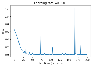
# plot the cost
plt.plot(np.squeeze(costs))
plt.ylabel('cost')
plt.xlabel('iterations (per tens)')
plt.title("Learning rate =" + str(learning_rate))
plt.show()
# lets save the parameters in a variable
parameters = sess.run(parameters)
print ("Parameters have been trained!")
# Calculate the correct predictions
correct_prediction = tf.equal(tf.argmax(Z3), tf.argmax(Y))
# Calculate accuracy on the test set
accuracy = tf.reduce_mean(tf.cast(correct_prediction, "float"))
print ("Train Accuracy:", accuracy.eval({X: X_train, Y: Y_train}))
print ("Test Accuracy:", accuracy.eval({X: X_test, Y: Y_test}))
# Save our trained model
saver = tf.train.Saver()
saver.save(sess, './TensorFlow-first-network')
return parametersRun the following cell to train our model. On my machine, it takes about 15 minutes, with GPU:
parameters = model(X_train, Y_train, X_test, Y_test)
Output:
Cost after epoch 100: 0.149014
Cost after epoch 200: 0.007334
Cost after epoch 300: 0.002902
Cost after epoch 400: 0.000667
Cost after epoch 500: 0.004335
Cost after epoch 600: 0.001176
Cost after epoch 700: 0.001851
Cost after epoch 800: 0.000289
Cost after epoch 900: 0.001448
Cost after epoch 1000: 0.000860
Parameters have been trained!
Train Accuracy: 1.0
Test Accuracy: 0.592
Amazing, our algorithm can recognize a cat and dog with 60% accuracy.
Insights:
- Our model seems big enough to fit the training set well. However, given the difference between train and test accuracy, we could try to add L2 or dropout regularization to reduce overfitting;
- Think about the session as a block of code to train the model. Each time we run the session on a minibatch, it trains the parameters. In total, we have run the session a large number of times (800 epochs) until we obtained well-trained parameters.
8 - Test with your own image:
We can now take a picture of our cat or dog and see the output of our model. To do that:
#test_image = "cat.jpg"
test_image = "dog.jpg"
my_image = read_image(test_image).reshape(1, ROWS*COLS*CHANNELS).T
X = my_image / 255.
print(X.shape)
Bellow we use predict function to predict Cat vs. Dog from our X image, we use our saved parameters:
def predict(X, parameters):

    W1 = tf.convert_to_tensor(parameters["W1"])
    b1 = tf.convert_to_tensor(parameters["b1"])
    W2 = tf.convert_to_tensor(parameters["W2"])
    b2 = tf.convert_to_tensor(parameters["b2"])
    W3 = tf.convert_to_tensor(parameters["W3"])
    b3 = tf.convert_to_tensor(parameters["b3"])

    params = {"W1": W1,
              "b1": b1,
              "W2": W2,
              "b2": b2,
              "W3": W3,
              "b3": b3}

    x = tf.placeholder("float", [X.shape[0], 1])

    z3 = forward_propagation(x, params)
    p = tf.argmax(z3)

    sess = tf.Session()
    prediction = sess.run(p, feed_dict = {x: X})

    return str(np.squeeze(prediction))

predict(X, parameters)
Output: '1'
9 - Restore the graph from the .meta file:
When we save the variables, it creates a .meta file. This file contains the graph structure. Therefore, we can import the meta graph using tf.train.import_meta_graph() and restore the values of the graph. Let's import the graph and see all tensors in the graph:
# delete the current graph
tf.reset_default_graph()

# import the graph from the file
imported_graph = tf.train.import_meta_graph('TensorFlow-first-network.meta')

# list all the tensors in the graph
for tensor in tf.get_default_graph().get_operations():
    print (tensor.name)
Output:
X
Y
W1/Initializer/random_uniform/shape
W1/Initializer/random_uniform/min
W1/Initializer/random_uniform/max
...
tf.train.Saver() saves the variables with the TensorFlow name. Now that we have the imported graph, we know that we are interested in W1... and b1... tensors; we can restore the parameters:
tf.reset_default_graph()
with tf.Session() as sess:

    ## Load the entire model previuosly saved in a checkpoint
    the_Saver = tf.train.import_meta_graph('TensorFlow-first-network' + '.meta')
    the_Saver.restore(sess, './TensorFlow-first-network')

    W1,b1,W2,b2,W3,b3 = sess.run(['W1:0', 'b1:0','W2:0','b2:0', 'W3:0','b3:0'])
    parameters = {"W1": W1,
              "b1": b1,
              "W2": W2,
              "b2": b2,
              "W3": W3,
              "b3": b3}
    #print("W1 = ", parameters["W1"])
    #print("b1 = ", parameters["b1"])
    #print("W2 = ", parameters["W2"])
    #print("b2 = ", parameters["b2"])
    #print("W3 = ", parameters["W3"])
    #print("b3 = ", parameters["b3"])
Now let's try again to predict our image, but now we will use parameters restored from our trained model:
predict(X, parameters)
Output: '1'
Conclusion:
So I should congratulate you on finishing your first deep network with the Tensorflow framework. What we should remember from this tutorial:
- Tensorflow is a programming framework used in deep learning;
- The two main object classes in TensorFlow are Tensors and Operators;
- When we code in TensorFlow, we have to take the following steps:
- Create a graph containing Tensors (Variables, Placeholders ...) and Operations (
tf.matmul, tf.add, ...); - Create a session;
- Initialize the session;
- Run the session to execute the graph;
- Create a graph containing Tensors (Variables, Placeholders ...) and Operations (
- We can execute the graph multiple times as you've seen in
model(); - The backpropagation and optimization are automatically done when running the session on the "optimizer" object.
In the next tutorial part, instead of using simple deep networks, we will use convolutional networks. You will see what difference we get! Full tutorial code and cats vs dogs image data-set can be found on my GitHub page.