OpenCV image stitching introduction

You probably already know that the Google Photos app has unique auto features like video creation, panoramic image stitching, image collage creation, image sorting, and more. Have you ever wondered how all these features work? So I thought about how difficult it can be to do a panorama merging on my own using the Python language.

So what is image stitching? The output is a composite image such that it is a culmination of image scenes. In simple terms, for input, there should be a group of pictures, but at the same time, the logical flow between the images must be preserved.

For example, think about the sea horizon while you are taking few photos of it. We essentially create a single stitched image from a group of these images that explains the entire scene in detail. It is quite an interesting algorithm.

Let's first understand the concept of image stitching. If you want to capture a big scene and your camera can only provide an image of a specific resolution and that resolution is 640 by 480, it is certainly not enough to capture the big panoramic view. So, we can capture multiple images of the entire scene and then put all bits and pieces together into one big picture. Such photos of ordered scenes of collections area units refer to as panoramas. The entire process of acquiring multiple images and merging them into such panoramas is named image stitching. And finally, we have one beautiful big and a large photograph of the scenic view.

First, we'll install OpenCV version 3.4.2.16. If you have a newer version, first do pip uninstall opencv before installing an older version. If you work with a more recent version, you will be required to build an OpenCV library by yourself to enable the image stitching function, so it's much easier to install an older version:

pip install opencv-contrib-python==3.4.2.16

import cv2
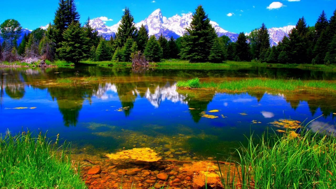
import numpy as np

We are taking this beautiful photo for our tutorial, which we will slice into two left and right images, and we'll try to get the same or very similar image back.

So here is the list of steps that we should do to get our final stitched result:

1. Calculate the key points and descriptions for sifting for both images;
2. Calculate the distances between each image descriptor and another image descriptor;
3. Select the top matches for each image descriptor;
4. To evaluate homography, run RANSAC;
5. Alight overlapping;
6. Now stitch them.

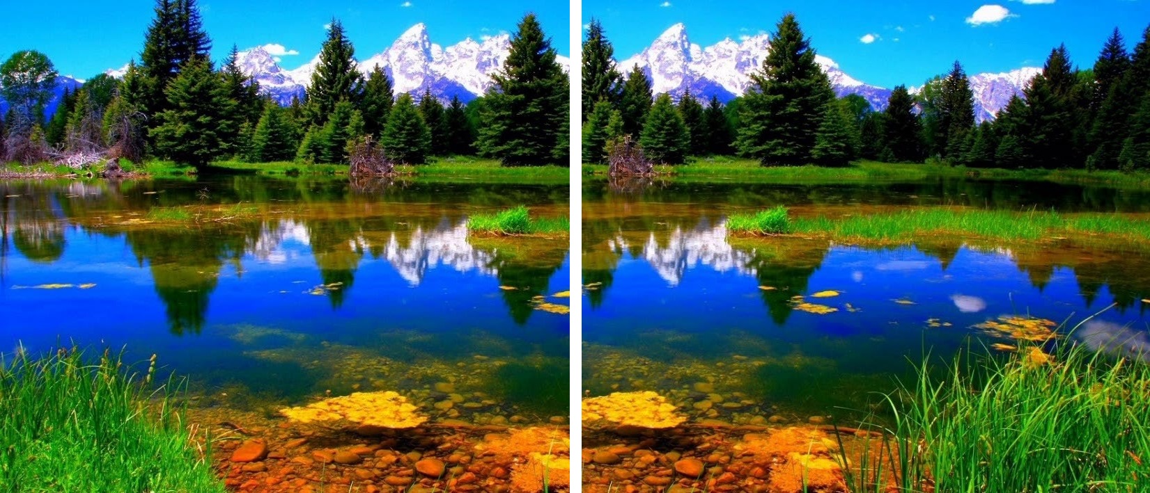
So starting from the first step, we are importing these two images and converting them to grayscale. If you are using large images, I recommend you to use cv2.resize because if you have an older computer, it may be prolonged and take quite some time. If you want to resize image size, i.e., by 50%, change from fx=1 to fx=0.5.

img_ = cv2.imread('original_image_left.jpg')
img_ = cv2.resize(img_, (0,0), fx=1, fy=1)
img1 = cv2.cvtColor(img_,cv2.COLOR_BGR2GRAY)

img = cv2.imread('original_image_right.jpg')
img = cv2.resize(img, (0,0), fx=1, fy=1)
img2 = cv2.cvtColor(img,cv2.COLOR_BGR2GRAY)

We still need to figure out the features that match both photos. We shall be using opencv_contrib'sopencv_contrib's SIFT descriptor. SIFT (Scale Invariant Feature Transform) is a very powerful OpenCV algorithm. You can read more OpenCV'sOpenCV's docs on SIFT for Image to understand more about features. These best-matched properties are the basics for image stitching. We distinguish the main points and descriptions of both images as follows:

sift = cv2.xfeatures2d.SIFT_create()
# find the key points and descriptors with SIFT
kp1, des1 = sift.detectAndCompute(img1,None)
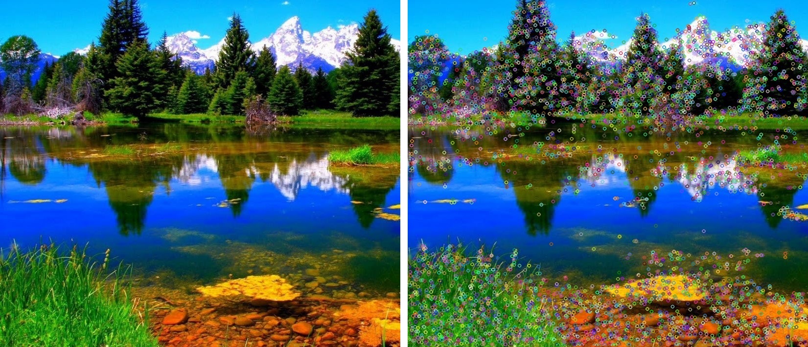
kp2, des2 = sift.detectAndCompute(img2,None)

kp1 and kp2 are the main points, des1 and des2 are the descriptions of the respective images. If we display this image with features, it will look like this:

cv2.imshow('original_image_left_keypoints',cv2.drawKeypoints(img_,kp1,None))

The image on the left shows the actual image. The image on the right is annotated with features detected by SIFT:

To match images can be used either FLANN or BFMatcher methods that OpenCV provides. I will write both examples to prove that we'll get the same result. Both examples do an image matching and find features that are most similar in both photos. If we set, for example, the parameter k = 2, we ask knnMatcher to return the two best matches for every descriptor. These "Matches" return lists in which each subgroup consists of "k" objects. To learn more about it, go here. And here is the code:

FLANN matcher code:

FLANN_INDEX_KDTREE = 0
index_params = dict(algorithm = FLANN_INDEX_KDTREE, trees = 5)
search_params = dict(checks = 50)
match = cv2.FlannBasedMatcher(index_params, search_params)
matches = match.knnMatch(des1,des2,k=2)

BFMatcher matcher code:

match = cv2.BFMatcher()
matches = match.knnMatch(des1,des2,k=2)

Often, there can be many possibilities in images that can exist in many places in the image. To solve this, we filter all matches found to get the best ones. To do that, we apply a test ratio using the two best matches we obtained above. We decide that we found a match if the ratio defined below is more significant than we specified.

good = []
for m,n in matches:
    if m.distance < 0.03*n.distance:
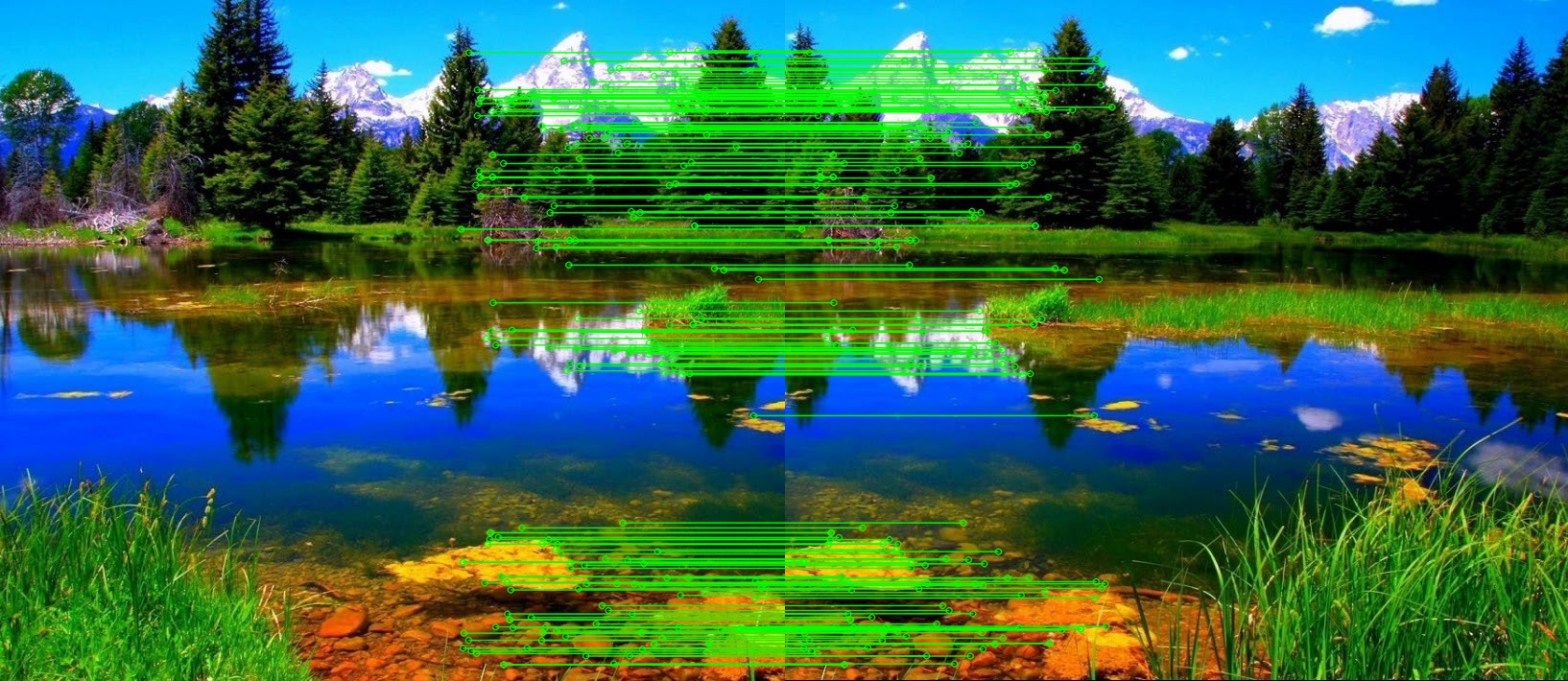
        good.append(m)

Now we are defining the parameters of drawing lines on the image and giving the output to see how it looks like when we found all matches on the image:

draw_params = dict(matchColor = (0,255,0), # draw matches in green color
                   singlePointColor = None,
                   flags = 2)

img3 = cv2.drawMatches(img_,kp1,img,kp2,good,None,**draw_params)
cv2.imshow("original_image_drawMatches.jpg", img3)

And here is the output image with matches drawn:

Here is the complete code of this tutorial up to this:

import cv2
import numpy as np

img_ = cv2.imread('original_image_left.jpg')
#img_ = cv2.resize(img_, (0,0), fx=1, fy=1)
img1 = cv2.cvtColor(img_,cv2.COLOR_BGR2GRAY)

img = cv2.imread('original_image_right.jpg')
#img = cv2.resize(img, (0,0), fx=1, fy=1)
img2 = cv2.cvtColor(img,cv2.COLOR_BGR2GRAY)

sift = cv2.xfeatures2d.SIFT_create()
# find the key points and descriptors with SIFT
kp1, des1 = sift.detectAndCompute(img1,None)
kp2, des2 = sift.detectAndCompute(img2,None)
#cv2.imshow('original_image_left_keypoints',cv2.drawKeypoints(img_,kp1,None))

#FLANN_INDEX_KDTREE = 0
#index_params = dict(algorithm = FLANN_INDEX_KDTREE, trees = 5)
#search_params = dict(checks = 50)
#match = cv2.FlannBasedMatcher(index_params, search_params)
match = cv2.BFMatcher()
matches = match.knnMatch(des1,des2,k=2)

good = []
for m,n in matches:
    if m.distance < 0.03*n.distance:
        good.append(m)

draw_params = dict(matchColor = (0,255,0), # draw matches in green color
                   singlePointColor = None,
                   flags = 2)

img3 = cv2.drawMatches(img_,kp1,img,kp2,good,None,**draw_params)
cv2.imshow("original_image_drawMatches.jpg", img3)

Conclusion:

So now, in this short tutorial, we finished 1–3 steps we wrote above, so 3 more steps left to do. So in the next tutorial, we’ll find homography for image transformation. Then we’ll be able to proceed with image stitching.