YOLOv3 theory explained

In this tutorial, I will explain what the YOLO model is and how it works in detail.

Tutorial content:

• What is Yolo?
• Prerequisites
• A Fully Convolutional Neural Network
• Interpreting the output
• Anchor Boxes and Predictions
• Dimensions of the Bounding Box
• Objectness Score and Class Confidences
• Prediction across different scales
• Output Processing (Filtering with a threshold on class scores)
• Implementation

1. What is Yolo?

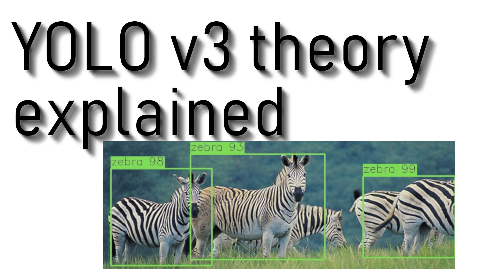
"You Only Look Once" is an algorithm that uses convolutional neural networks for object detection. You only look once, or YOLO is one of the faster object detection algorithms out there. Though it is not the most accurate object detection algorithm, it is an excellent choice when we need real-time detection without losing too much accuracy.

In comparison to recognition algorithms, a detection algorithm predicts class labels and detects objects locations. So, It not only classifies the image into a category, but it can also detect multiple Objects within an Image. This algorithm applies a single Neural network to the Full Image. It means that this Network divides the image into regions and predicts bounding boxes and probabilities for each area. The predicted probabilities weigh these bounding boxes.

The last time when I was working with object detection, I made a CS:GO aimbot tutorial, but it was pretty slow (~10 FPS). So now it's time to make it work faster. One of the biggest takeaways from this experience is realizing that the best way to learn an object detection algorithm is to implement it from scratch by yourself. That's a short introduction to what we'll do in this tutorial. But before we get out hands dirty with code, we must understand how YOLO works.

2. Prerequisites

To fully understand this tutorial:

• It would be best if you would have a basic understanding of how convolutional neural networks work. That includes knowledge of Residual Blocks, skip connections, and Upsampling;
• What does object detection means, what is bounding box regression, IoU, and non-maximum suppression;
• You should be able to create simple neural networks with ease.

3. A Fully Convolutional Neural Network

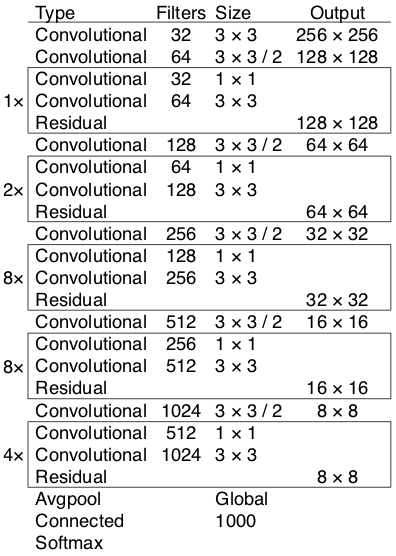
In the YOLO v3 paper, the authors present a new, more profound architecture of feature extractors called Darknet-53. Its name suggests that it contains 53 convolutional layers, each followed by batch normalization and Leaky ReLU activation. YOLO makes use of only convolutional layers, making it a fully convolutional network (FCN), so it can avoid of using pooling layers. Instead, a convolutional layer with a stride of two is used to downsample the feature maps. This helps to prevent the loss of low-level features attached to pooling layers.

YOLO is invariant to the size of the input image. However, in practice, we might want to stick to a regular input size due to various problems that only show their heads when implementing the algorithm.

A big one among these problems is that if we want to process our images in batches (images in clusters can be processed in parallel by the GPU, leading to speed boosts), we need to have all fixed height and width images. This is required to concatenate multiple images into a large batch.

The Network downsamples the image by a factor called the stride of the Network. Generally, the stride of any layer in the Network is equal to the factor by which the layer's output is smaller than the input image to the Network. For example, if the stride of the Network is 32, then an input image of size 416 x 416 will yield an output of size 13 x 13.

4. Interpreting the output

First things to know:

• The input is a batch of images of shape (m, 416, 416, 3);
• The output is a list of bounding boxes along with the recognized classes. Six numbers represent each bounding box (p_c, b_x, b_y, b_h, b_w, c). If we expand c into an 80-dimensional vector, each bounding box is then represented by 85 numbers.

In the same way, as in all object detectors, the features learned by the convolutional layers are passed onto a classifier/regressor, which makes the detection prediction (coordinates of the bounding boxes, the class label, etc.).

In YOLO, the prediction is made by using a convolutional layer that uses 1 x 1 convolutions. So, the first thing to notice is our output is a feature map. Since we have used 1 x 1 convolution, the size of the prediction map is exactly the size of the feature map before it. In YOLO v3, you interpret this prediction map because each cell can predict a fixed number of bounding boxes.

For example, we have (B x (5 + C)) entries in the feature map. B represents the number of bounding boxes each cell can predict. According to the paper, each of these B bounding boxes may specialize in detecting a certain kind of object. Each bounding box has 5 + C attributes, which describe the center coordinates, dimensions, objectness score, and C class confidences for each bounding box. YOLO v3 predicts three bounding boxes for every cell.

We expect each cell of the feature map to predict an object through one of its bounding boxes if the object's center falls in the receptive field of that cell.

This has to do with how YOLO is trained, where only one bounding box is responsible for detecting any given object. First, we must ascertain which of the cells this bounding box belongs to.

To do that, we divide the input image into a grid of dimensions equal to that of the final feature map. Take a look at the example below, where the input image is 416 x 416, and the stride of the Network is 32. As pointed earlier, the dimensions of the feature map will be 13 x 13. We then divide the input image into 13 x 13 cells.

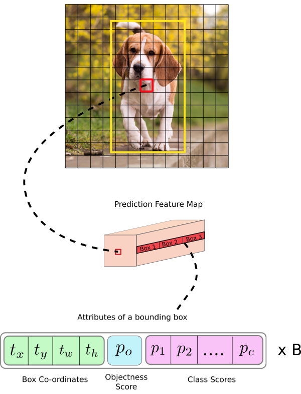Then, the cell (on the input image) containing the center of the ground truth box of an object is chosen to be the one responsible for predicting the object. The image is the cell marked red, which contains the center of the ground truth box (marked yellow).

Now, the red cell is the 7th cell in the 7th row on the grid. We now assign the 7th cell in the 7th row on the feature map (corresponding cell on the feature map) as the one responsible for detecting the dog.

Now, this cell can predict three bounding boxes. Which one will be assigned to the dog's ground truth label? To understand that, we must wrap our heads around the concept of anchors. (Note that the cell we're talking about here is a cell on the prediction feature map. We divide the input image into a grid to determine which cell of the prediction feature map is responsible for prediction)

For better understanding, we can analyze another example with more images:

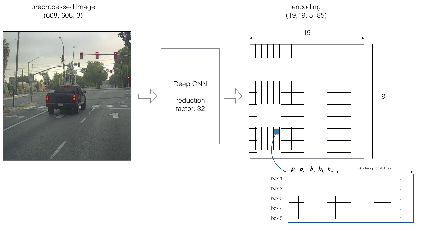
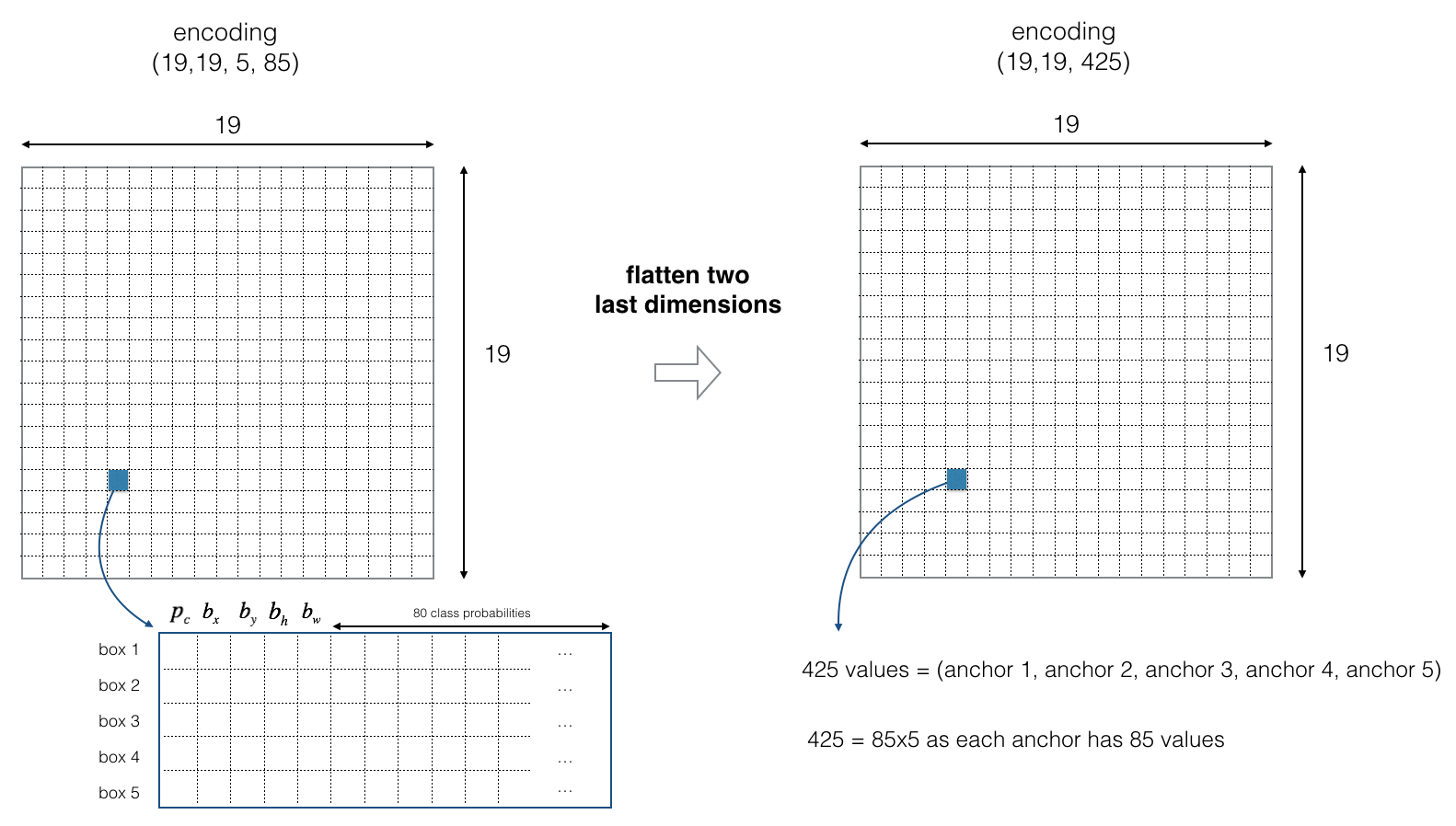
Now we will use five anchor boxes. So we can think of the YOLO architecture as the following: IMAGE (m, 608, 608, 3) -> DEEP CNN -> ENCODING (m, 19, 19, 5, 85). Someone may ask where this 19 number came from? Answer: the same way as before 608/32=19

Let's look in greater detail at what this encoding represents:

If the center/midpoint of an object falls into a grid cell, that grid cell is responsible for detecting that object.

Since we are using five anchor boxes, each of the 19x19 cells thus encodes information about five boxes. Anchor boxes are defined only by their width and height.

For simplicity, we will flatten the last two dimensions of the shape (19, 19, 5, 85) encoding. So the output of the Deep CNN is (19, 19, 425):

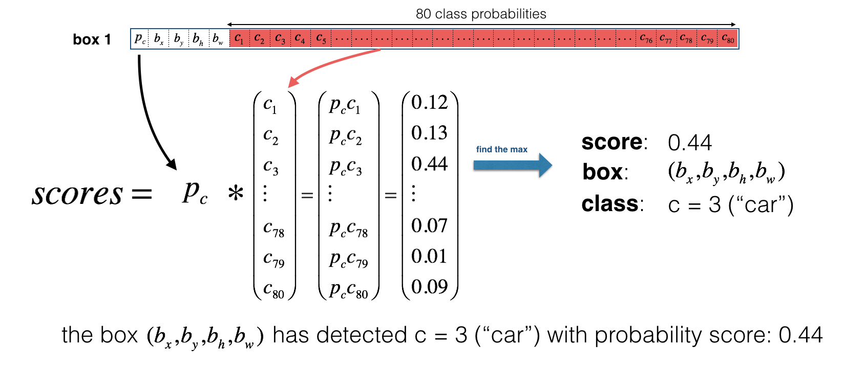
We will compute the following elementwise product for each box (of each cell) and extract a probability that the box contains a specific class.

Here's one way to visualize what YOLO is predicting on an image:

• For each of the 19x19 grid cells, find the maximum probability scores (taking a max across both the five anchor boxes and across different classes);
• Color that grid cell according to what object that grid cell considers the most likely.

Doing this results in this picture:

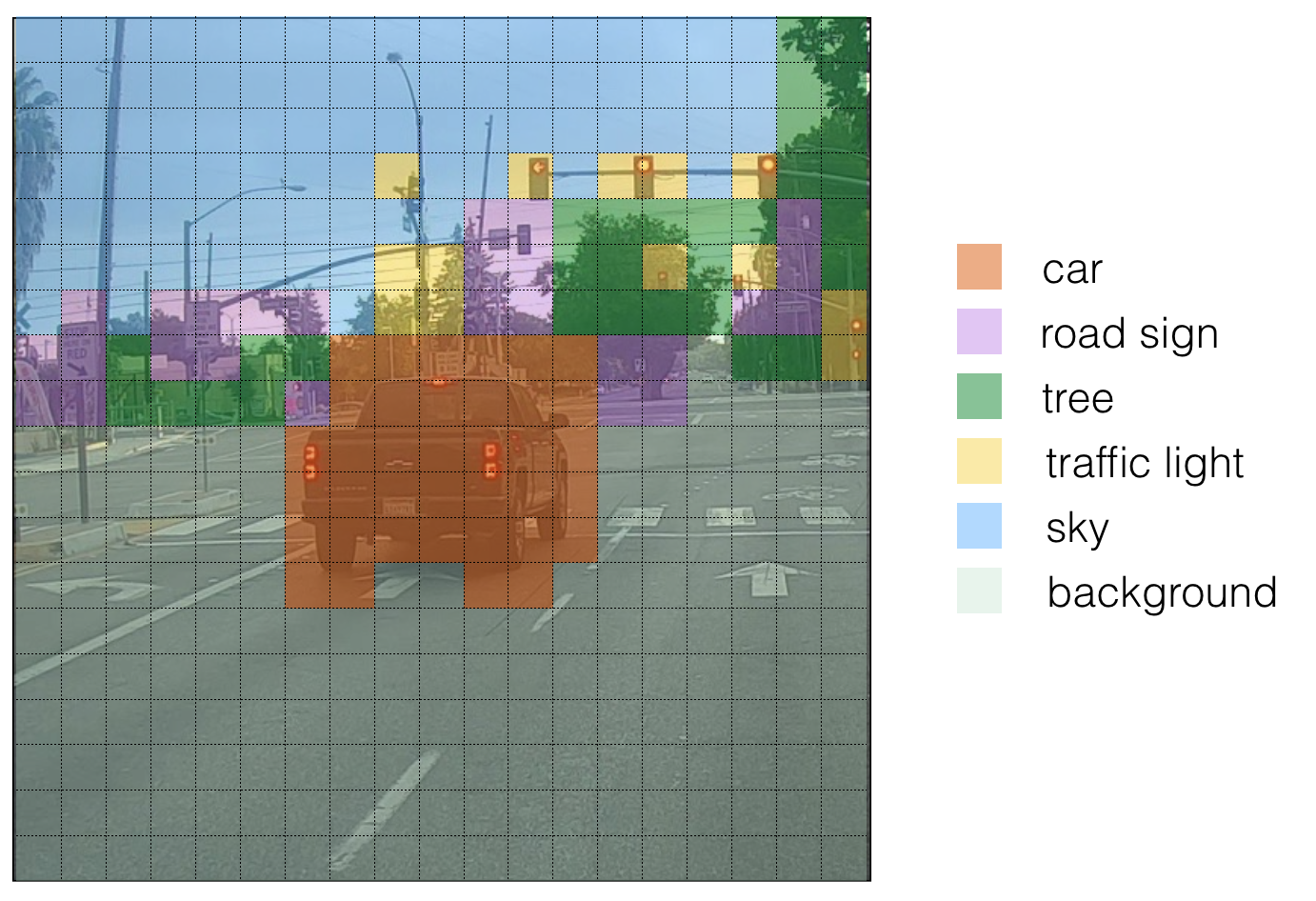The above visualization isn't a core part of the YOLO algorithm for making predictions; it's just an excellent way of visualizing an intermediate result of the algorithm.

Another way to visualize YOLO's output is to plot the bounding boxes that it outputs. Doing that results in a visualization like this:

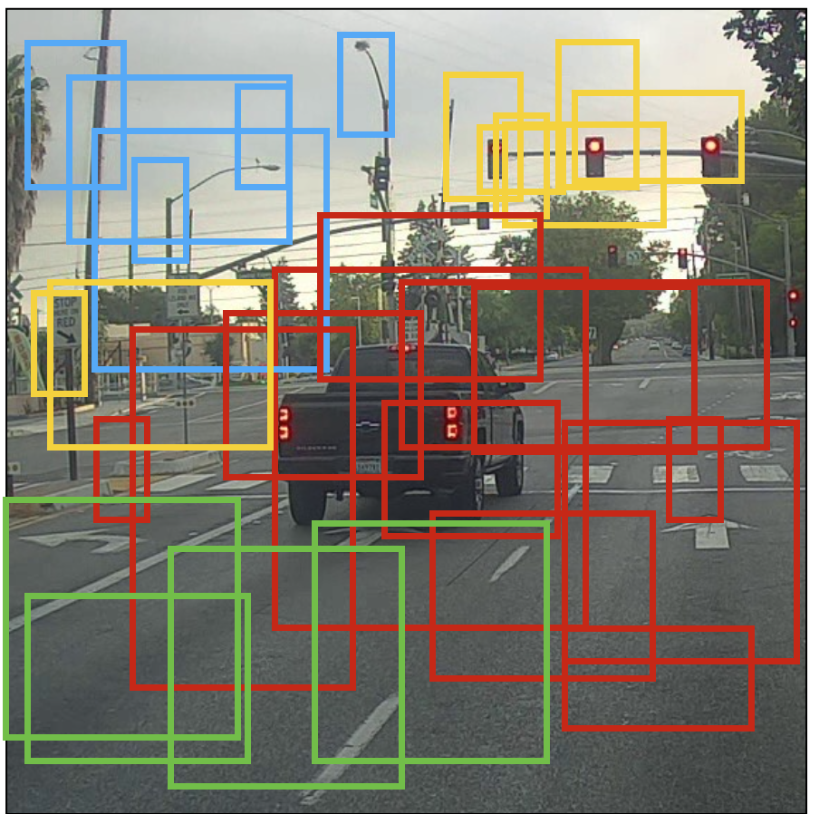
In the figure above, we plotted only boxes that the model had assigned a high probability to, but this is still too many boxes. We want to filter the algorithm's output down to a much smaller number of detected objects. To do so, we'll use non-max suppression, more about that, and we'll talk in 9th this tutorial part.

5. Anchor Boxes and Predictions

Predicting the bounding box's width and height might make sense, but that leads to unstable gradients during training. Instead, most modern object detectors predict log-space transforms or offsets to pre-defined default bounding boxes called anchors.

Then, these transforms are applied to the anchor boxes to obtain the prediction. YOLO v3 has three anchors, which result in the prediction of three bounding boxes per cell.

Anchors are bounding box priors that were calculated on the COCO dataset using k-means clustering. We are going to predict the width and height of the box as offsets from cluster centroids. The box's center coordinates relative to the location of the filter application are predicted using a sigmoid function.

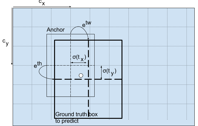
The following formula describes how the network output transformed to obtain bounding box predictions:

$$\begin{gathered} b_x=\sigma \left(t_x\right)+c_x \\ {b}_y=\sigma \left(t_y\right)+c_y \\ {b}_w=p_w{e}^{t_w} \\ {b}_h=p_h{e}^{t_h} \end{gathered}$$

Here b_x, b_y, b_w, b_h are the x, y center coordinates, width, and height of our prediction. t_x, t_y, t_w, t_h (xywh) is what the network outputs. c_x and c_y are the top-left coordinates of the grid. p_w and p_h are anchors dimensions for the box.

Center Coordinates

We are running our center coordinates prediction through a sigmoid function. This forces the value of the output to be between 0 and 1. Usually, YOLO doesn't predict the absolute coordinates of the bounding box's center. It predicts offsets which are:

• Relative to the top left corner of the grid cell, which is predicting the object;
• Normalized by the dimensions of the cell from the feature map, which is, 1.

For example, consider the case of our above dog image. If the prediction coordinates for the center are (0.4, 0.7), then this means that the center lies at (6.4, 6.7) on the 13 x 13 feature map. (Since the top-left coordinates of the red cell are (6,6)).

But wait, what happens if the predicted x and y coordinates are greater than one, for example (1.2, 0.7). This means that center lies at (7.2, 6.7). The center now lies in a cell just right to our red cell, or the 8th cell in the 7th row. This breaks the theory behind YOLO because if we postulate that the red box is responsible for predicting the dog, the center of the dog must lie in the red cell and not in the one beside it. So, to solve this problem, the output is passed through a sigmoid function, which squashes the output in a range from 0 to 1, effectively keeping the center in the grid which is predicting.

6. Dimensions of the Bounding Box

The dimensions of the bounding box are predicted by applying a log-space transformation to the output and then multiplying with an anchor.

Here predictions, b_w, and b_h, are normalized by the height and width of the image. (Training labels are chosen this way). So, if the predictions b_x and b_y for the box containing the dog are (0.3, 0.8), then the actual width and height on the 13 x 13 feature map are (13∗0.3, 13∗0.8).

7. Objectness Score and Class Confidences

Fir of all, the object score represents the probability that an object contains inside a bounding box. It should be nearly 1 for the red and the neighboring grids, whereas almost 0 for the grid at the corners.

The objectness score is also passed through a sigmoid, which should we can interpret as a probability.

Talking about Class confidences, they represent the probabilities of the detected object belonging to a particular class (Dog, Cat, person, car, bicycle, etc.). In older YOLO versions, the softmax activation function was used to calculate the class scores.

In YOLO, authors have decided to use sigmoid instead. The reason is that Softmaxing class scores assume that the classes are mutually exclusive. In simple words, if an object belongs to one class, then it cannot belong to another class. This is true for the COCO database, which we will implement first.

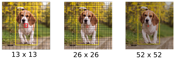
8. Prediction across different scales

YOLO v3 predicts three different scales. The detection layer is used to detect feature maps of three different sizes, having strides 32, 16, 8, respectively. This means that with an input of 416 x 416, we make detections on scales 13 x 13, 26 x 26, and 52 x 52.

The Network downsamples the input image until the first detection layer, where detection is made using feature maps of a layer with stride 32. Further, layers are upsampled by a factor of 2 and concatenated with feature maps of a previous layer having identical feature map sizes. Another detection is now made at layer with stride 16. The same upsampling procedure is repeated, and a final detection is made at the layer of stride 8.

Each cell predicts three bounding boxes using three given anchors at each scale, making the total number of anchors used 9. (The anchors are different for different scales).

YOLO authors report that this helps better detect tiny objects; this was a frequent complaint with the earlier YOLO versions. Upsampling helps the Network to learn fine-grained features that are instrumental for detecting small objects.

9. Output Processing (Filtering with a threshold on class scores)

For an image of size 416 x 416, YOLO predicts ((52 x 52) + (26 x 26) + 13 x 13)) x 3 = 10647 bounding boxes. However, in the case of our image, there's only one object, a dog. So, you may ask, how do we reduce the detections from 10647 to 1?

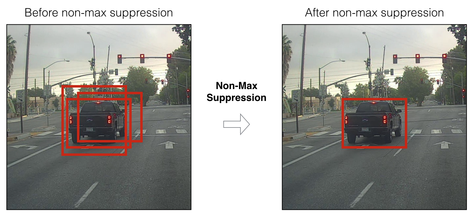
First, we filter boxes based on their objectness score. Generally, boxes having scores below a threshold (for example, below 0.5) are ignored. Next, Non-maximum Suppression (NMS) intends to cure the problem of multiple detections of the same image. For example, all the three bounding boxes of the red grid cell may detect a box, or the adjacent cells may detect the same object, so NMS is used to remove multiple detections.

Specifically, we'll carry out these steps:

• Get rid of boxes with a low score (meaning, the box is not very confident about detecting a class);
• Select only one box when several boxes overlap and detect the same object (Non-max suppression).

For better understanding, I will use the same example with a car I mentioned above. At first, we are going to apply the first filter by thresholding. We want to get rid of any box for which the class "score" is less than a chosen threshold. The model gives us a total of 19x19x5x85 numbers, with each box described by 85 numbers. It'll be convenient to rearrange the (19,19,5,85) (or (19,19,425)) dimensional tensor into the following variables:

• box_confidence: tensor of shape (19×19,5,1) containing p_c (confidence probability that there's some object) for each of the 5 boxes predicted in each of the 19x19 cells;
• boxes: tensor of shape (19×19,5,4) containing (b_x, b_y, b_h, b_w) for each of the 5 boxes per cell;
• box_class_probs: tensor of shape (19×19,5,80) containing the detection probabilities (c₁, c₂, ..., c₈₀) for each of the 80 classes for each of the 5 boxes per cell.

Even after filtering by thresholding over the classes scores, we still end up with many overlapping boxes. A second filter for selecting the right boxes is called NMS. NMS uses the critical function called "Intersection over Union", or IoU.

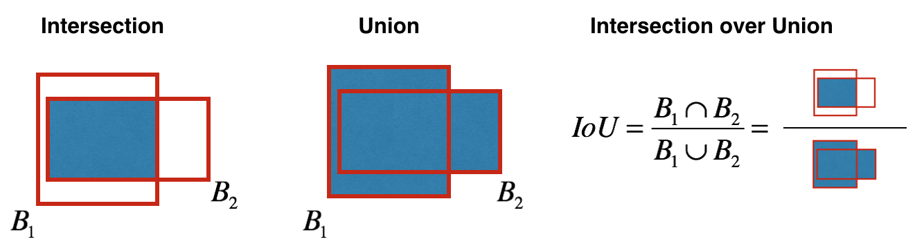Implementing IoU:

• So we define a box using its two corners (upper left and lower right): (x1, y1, x2, y2) rather than the midpoint and height/width;
• To calculate the area of a rectangle, we need to multiply its height (y2 - y1) by its width (x2 - x1);
• We also need to find the coordinates (xi1, yi1, xi2, yi2) of the intersection of two boxes:
• xi1 = maximum of the x1 coordinates of the two boxes;
• yi1 = maximum of the y1 coordinates of the two boxes;
• xi2 = minimum of the x2 coordinates of the two boxes;
• yi2 = minimum of the y2 coordinates of the two boxes;

Arguments:
box1 - first box, list object with coordinates (x1, y1, x2, y2);
box2 - second box, list object with coordinates (x1, y1, x2, y2).

xi1 = max(box1[0], box2[0])
yi1 = max(box1[1], box2[1])
xi2 = min(box1[2], box2[2])
yi2 = min(box1[3], box2[3])
inter_area = (xi2 - xi1)*(yi2 - yi1)

# Formula: Union(A,B) = A + B - Inter(A,B)
box1_area = (box1[3] - box1[1])*(box1[2]- box1[0])
box2_area = (box2[3] - box2[1])*(box2[2]- box2[0])
union_area = (box1_area + box2_area) - inter_area

# compute the IoU
IoU = inter_area / union_area

Now, to implement non-max suppression, the key steps are:

• Select the box that has the highest score;
• Compute its overlap with all other boxes, and remove boxes that overlap it more than iou_threshold;
• Go back to step 1 and iterate until there are no more boxes with a lower score than the selected box.

These steps will remove all boxes that have a large overlap with the selected boxes. Only the "best" boxes remain:

10. Implementation

YOLO can only detect objects belonging to the classes present in the dataset used to train the Network. I will be using the official weight file for our detector. These weights have been obtained by training the Network on the COCO dataset, and therefore we can detect 80 object categories.

Here one more time, I will come back to my example with a car to summarise how our model should work:

• Input image (608, 608, 3);
• The input image goes through a CNN, resulting in a (19,19,5,85) dimensional output;
• After flattening the last two dimensions, the output is a volume of shape (19, 19, 425):
• Each cell in a 19x19 grid over the input image gives 425 numbers;
• 425 = 5 x 85 because each cell contains predictions for five boxes, corresponding to 5 anchor boxes;
• 85 = 5 + 80, where five is because (p_c, b_x ,b_y, b_h, b_w) has five numbers, and 80 is the number of classes we set to detect.
• Next, select only a few boxes based on:
• Score-thresholding: throws away boxes that have detected a class with a score less than the threshold;
• Non-max suppression: Compute the Intersection over Union and avoid selecting overlapping boxes.
• This gives us YOLO's final output.

Conclusion:

That's it for the theory part. I explained enough about the YOLO algorithm to understand how it works. In the next part, I will implement various layers required to run YOLOv3 with TensorFlow.