Understanding Logistic Regression Sigmoid function

To learn about Logistic Regression, at first, we need to learn Logistic Regression basic properties. Only then will we be able to build a machine learning model on a real-world application. So we will do everything step by step.

Classification techniques are an essential part of machine learning and data mining applications. Most problems in Data Science are classification problems. There are many classification problems available, but logistics regression is common and is a useful regression method for solving binary classification problems.

Logistic Regression can be used for various classification problems such as spam detection, prediction if a customer will purchase a particular product or choosing another competitor, whether the user will click on a given advertisement link or not, and many more examples.

Logistic Regression is one of the most simple and commonly used Machine Learning algorithms for two-class classification. It is easy to implement and can be used as the baseline for any binary classification problem. Its basic fundamental concepts are also constructive in deep learning. Logistic regression describes and estimates the relationship between one dependent binary variable and independent variables.

Numpy is the main and the most used package for scientific computing in Python. It is maintained by a large community (www.numpy.org). In this tutorial, we will learn several key NumPy functions such as np.exp and np.reshape. You will need to know how to use these functions for future deep learning tutorials.

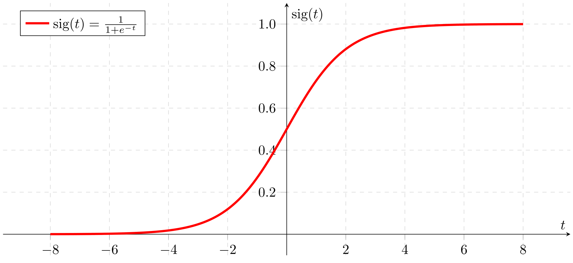
At first, we must learn to implement a sigmoid function. It is a logistic function that gives an ‘S’ shaped curve that can take any real-valued number and map it into a value between 0 and 1. If the curve goes to positive infinity, y predicted will become 1, and if the curve goes to negative infinity, y predicted will become 0. If the output of the sigmoid function is more than 0.5, we can classify the outcome as 1 or YES, and if it is less than 0.5, we can classify it as 0 or NO. For example: If the output is 0.75, we can say in terms of the probability that there is a 75 percent chance that the patient will have cancer.

Before using np.exp(), you will use math.exp() to implement the sigmoid function. You will then see why np.exp() is preferable to math.exp(). So here is the sigmoid activation function:

$f\left(x\right)=\frac{1}{1+e^{-x}}$

Sigmoid is also known as the logistic function. It is a non-linear function used in Machine Learning (Logistic Regression) and Deep Learning. The sigmoid function curve looks like an S-shape:

Let's write the code to see an example with math.exp().

import math

def basic_sigmoid(x):
    s = 1/(1+math.exp(-x))
    return s

Let's try to run the above function: basic_sigmoid(1). As a result, we should receive "0.7310585786300049".

Actually, we rarely use the "math" library in deep learning because the functions' inputs are real numbers. In deep learning, we mostly use matrices and vectors. This is why NumPy is more powerful and useful. For example, if we'll try to run a list into the above function:

x = [1, 2, 3]
print(basic_sigmoid(x))

If we run the above code, we will receive an error about a bad operand. If we would like to run such lists, we would need to modify our basic_sigmoid() function, inserting for loop, but then losing computation power. So, in this case, we'll write a sigmoid function to use vectors instead of scalars:

import numpy as np

def sigmoid(x):
    s = 1/(1+np.exp(-x)) 
    return s

x could now be either a real number, a vector, or a matrix. Data structures we use in NumPy to represent these shapes are vectors or matrices called NumPy arrays. Now we can call, for example, this function:

x = np.array([3, 2, 1])
print(sigmoid(x))

As a result, we should see: "[0.95257413 0.88079708 0.73105858]".

When constructing Neural Network (NN) models, one of the primary considerations is choosing activation functions for hidden and differentiable output layers. This is because calculating the backpropagated error signal used to determine NN parameter updates requires the gradient of the activation function gradient. Three of the most commonly-used activation functions used in NNs are the relu function, the logistic sigmoid function, and the tangent function. Simply talking, we need to compute gradients to optimize loss functions using backpropagation. Let's code your first sigmoid gradient function:

$sigmoid\_derivative\left(x\right)=\sigma \text{'}\left(x\right)=\sigma \left(x\right)·(1-\sigma (x\left)\right)$

We'll code the above function in two steps:
1. Set s to be the sigmoid of x. we'll use sigmoid(x) function.
2. Then we compute σ′(x)=s(1−s):

import numpy as np

def sigmoid_derivative(x):
    s = sigmoid(x)
    ds = s*(1-s)
    return ds

Above, we compute the gradient (also called the slope or derivative) of the sigmoid function concerning its input x. We can store the output of the sigmoid function into variables and then use it to calculate the gradient.
Let's test our code:

x = np.array([3, 2, 1])
print(sigmoid_derivative(x))

As a result, we receive "[0.04517666 0.10499359 0.19661193]"

To visualize our sigmoid and sigmoid_derivative functions, we can generate data from -10 to 10 and use matplotlib to plot these functions. Below is the full code used to print sigmoid and sigmoid_derivative functions:

from matplotlib import pylab
import pylab as plt
import numpy as np

def sigmoid(x):
    s = 1/(1+np.exp(-x))   
    return s

def sigmoid_derivative(x):
    s = sigmoid(x)
    ds = s*(1-s)
    return ds

# linespace generate an array from start and stop value, 100 elements
values = plt.linspace(-10,10,100)

# prepare the plot, associate the color r(ed) or b(lue) and the label 
plt.plot(values, sigmoid(values), 'r')
plt.plot(values, sigmoid_derivative(values), 'b')

# Draw the grid line in background.
plt.grid()

# Title & Subtitle
plt.title('Sigmoid and Sigmoid derivative functions')

# plt.plot(x)
plt.xlabel('X Axis')
plt.ylabel('Y Axis')

# create the graph
plt.show()

As a result, we receive the following graph:

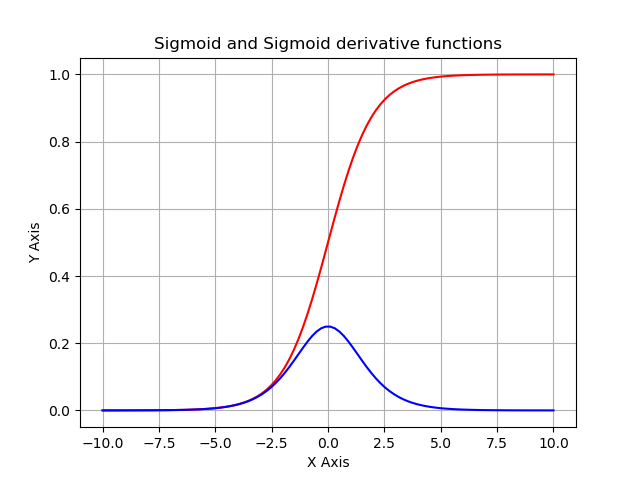
The above curve in red is a plot of our sigmoid function, and the curve in red color is our sigmoid_derivative function.

Conclusion: