Logistic Regressions architecture of the learning rate

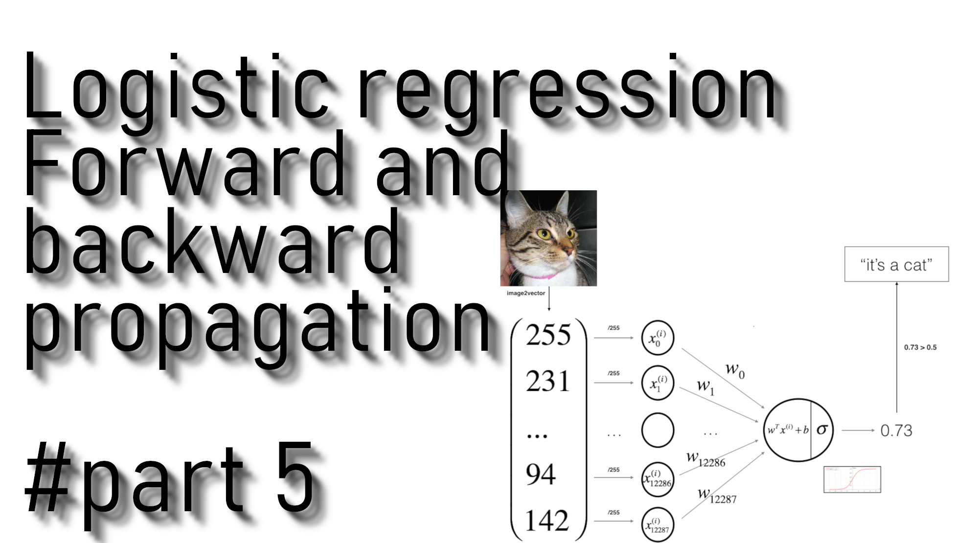
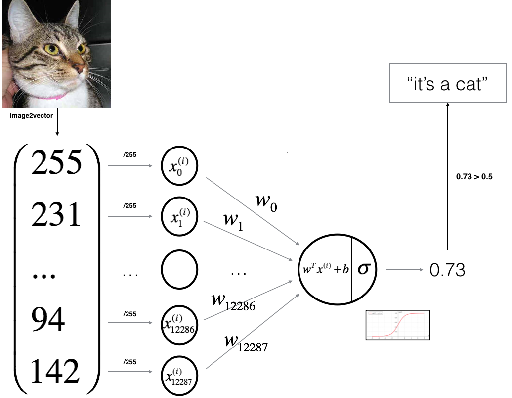
In this part, we'll design a simple algorithm to distinguish cat images from dog images. We will build a Logistic Regression using a Neural Network mindset. Figure bellow explains why Logistic Regression is actually a very simple Neural Network (one neuron):

Parts of our algorithm:

The main steps we will use to build a "Neural Network" are:

• Define the model structure (data shape).
• Initialize model parameters.
• Learn the parameters for the model by minimizing the cost:
  - Calculate current loss (forward propagation).
  - Calculate current gradient (backward propagation).
  - Update parameters (gradient descent).
• Use the learned parameters to make predictions (on the test set).
• Analyse the results and conclude the tutorial.

We will build the above parts separately, and then we will integrate them into one function called model().

In our first tutorial part, we already wrote a sigmoid function so that I will copy it from there:

def sigmoid(z):
	s = 1/(1+np.exp(-z))
	return s

Forward propagation:

First, weight and bias values are propagated forward through the model to arrive at a predicted output. At each neuron/node, the linear combination of the inputs is then multiplied by an activation function — the sigmoid function in our example. In this process, weights and biases are propagated from inputs to output is called forward propagation. After arriving at the predicted output, the loss for the training example is calculated.

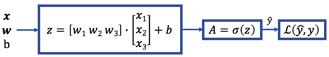
The mathematical expression of the forward propagation algorithm for one example:

Then the cost is computed by summing over all training examples:

And our final forward propagation cost function will look like this:

Backward propagation:

Backpropagation is the process of calculating the partial derivatives from the loss function back to the inputs. We are updating the values of w and b that lead us to the minimum. It’s helpful to write out the partial derivatives starting from dA to see how to arrive at dw and db.

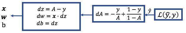
The mathematical expression of backward propagation (calculating derivatives):

Coding forward and backward propagation:

So we will implement the function explained above, but first, let's see what the inputs and outputs are:

Arguments:

w - weights, a NumPy array of size (ROWS * COLS * CHANNELS, 1);
b - bias, a scalar;
X - data of size (ROWS * COLS * CHANNELS, number of examples);
Y - true "label" vector (containing 0 if a dog, 1 if cat) of size (1, number of examples).

Return:

cost - cost for logistic regression;
dw - gradient of the loss with respect to w, the same shape as w;
db - gradient of the loss with respect to b, the same shape as b.

Here is the code we wrote in the video tutorial:

def propagate(w, b, X, Y):
    m = X.shape[1]
    
     # FORWARD PROPAGATION (FROM X TO COST)
    z = np.dot(w.T, X)+b # tag 1
    A = sigmoid(z) # tag 2                                    
    cost = (-np.sum(Y*np.log(A)+(1-Y)*np.log(1-A)))/m # tag 5
    
    # BACKWARD PROPAGATION (TO FIND GRAD)
    dw = (np.dot(X,(A-Y).T))/m # tag 6
    db = np.average(A-Y) # tag 7

    cost = np.squeeze(cost)
    grads = {"dw": dw,
             "db": db}
    
    return grads, cost

Let's test the above function with sample data:

w = np.array([[1.],[2.]])
b = 4.
X = np.array([[5., 6., -7.],[8., 9., -10.]])
Y = np.array([[1,0,1]])

grads, cost = propagate(w, b, X, Y)
print ("dw = " + str(grads["dw"]))
print ("db = " + str(grads["db"]))
print ("cost = " + str(cost))

As a result, you should get:

dw = [[4.33333333]
 [6.33333333]]
db = 2.934645119504845e-11
cost = 16.999996678946573

Full tutorial code:

import os
import cv2
import numpy as np
import matplotlib.pyplot as plt
import scipy

ROWS = 64
COLS = 64
CHANNELS = 3

TRAIN_DIR = 'Train_data/'
TEST_DIR = 'Test_data/'

train_images = [TRAIN_DIR+i for i in os.listdir(TRAIN_DIR)]
test_images =  [TEST_DIR+i for i in os.listdir(TEST_DIR)]

def read_image(file_path):
	img = cv2.imread(file_path, cv2.IMREAD_COLOR)
	return cv2.resize(img, (ROWS, COLS), interpolation=cv2.INTER_CUBIC)

def prepare_data(images):
	m = len(images)
	X = np.zeros((m, ROWS, COLS, CHANNELS), dtype=np.uint8)
	y = np.zeros((1, m))
	for i, image_file in enumerate(images):
		X[i,:] = read_image(image_file)
		if 'dog' in image_file.lower():
			y[0, i] = 1
		elif 'cat' in image_file.lower():
			y[0, i] = 0
	return X, y

train_set_x, train_set_y = prepare_data(train_images)
test_set_x, test_set_y = prepare_data(test_images)

train_set_x_flatten = train_set_x.reshape(train_set_x.shape[0], ROWS*COLS*CHANNELS).T
test_set_x_flatten = test_set_x.reshape(test_set_x.shape[0], -1).T
'''
print("train_set_x shape " + str(train_set_x.shape))
print("train_set_x_flatten shape: " + str(train_set_x_flatten.shape))
print("train_set_y shape: " + str(train_set_y.shape))
print("test_set_x shape " + str(test_set_x.shape))
print("test_set_x_flatten shape: " + str(test_set_x_flatten.shape))
print("test_set_y shape: " + str(test_set_y.shape))
'''
train_set_x = train_set_x_flatten/255
test_set_x = test_set_x_flatten/255

def sigmoid(z):
    s = 1/(1+np.exp(-z))
    return s

def propagate(w, b, X, Y):
    m = X.shape[1]
    
     # FORWARD PROPAGATION (FROM X TO COST)
    z = np.dot(w.T, X)+b
    A = sigmoid(z)                                    
    cost = (-np.sum(Y*np.log(A)+(1-Y)*np.log(1-A)))/m
    
    # BACKWARD PROPAGATION (TO FIND GRAD)
    dw = (np.dot(X,(A-Y).T))/m
    db = np.average(A-Y)

    cost = np.squeeze(cost)
    grads = {"dw": dw,
             "db": db}
    
    return grads, cost


w = np.array([[1.],[2.]])
b = 4.
X = np.array([[5., 6., -7.],[8., 9., -10.]])
Y = np.array([[1,0,1]])

grads, cost = propagate(w, b, X, Y)
print ("dw = " + str(grads["dw"]))
print ("db = " + str(grads["db"]))
print ("cost = " + str(cost))