Reshaping arrays, normalizing rows and softmax function in machine learning

In the previous tutorial, we learned how to code Sigmoid and Sigmoid gradient functions. In this tutorial, we'll learn how to reshape arrays, normalize rows, what is broadcasting, and softmax.

Two common NumPy functions used in deep learning are np.shape and np.reshape(). The shape function is used to get the shape (dimension) of a matrix or vector X. Reshape(...) is used to reshape the matrix or vector into another dimension.

For example, in computer science, a standard image is represented by a 3D array of shape (length, height, depth). However, when you read an image as the input of an algorithm, you convert it to a vector of shape (length*height*depth,1). In other words, you "unroll", or reshape, the 3D array into a 1D vector:

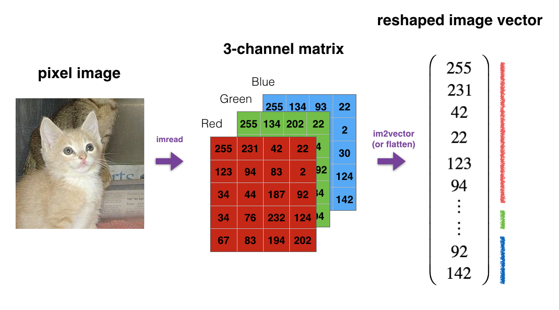
So we will implement a function that takes an input of shape (length, height, depth) and returns a vector of shape (length*height*depth,1). For example, if you would like to reshape an array A of shape (a, b, c) into a vector of shape (a*b,c), you would do:

A = A.reshape((A.shape[0]*A.shape[1], A.shape[2])) # A.shape[0] = a ; A.shape[1] = b ; A.shape[2] = c	

To implement the above function, we write simple few lines of code:

def image2vector(image):
    A = image.reshape( image.shape[0]*image.shape[1]*image.shape[2],1)
    return A	

To test our above function, we will create a 3 by 3 by 2 array. Typically images will be (num_px_x, num_px_y,3) where 3 represents the RGB values:

image = np.array([
    [[ 11,  12],
     [ 13,  14],
     [ 15,  16]],
    [[ 21,  22],
     [ 23,  24],
     [ 25,  26]],
    [[ 31,  32],
     [ 33,  34],
     [ 35,  36]]])

print(image2vector(image))
print(image.shape)	
print(image2vector(image).shape)

As a result, we will receive:

[[11]
 [12]
 [13]
 [14]
 [15]
 [16]
 [21]
 [22]
 [23]
 [24]
 [25]
 [26]
 [31]
 [32]
 [33]
 [34]
 [35]
 [36]]
(3, 3, 2)
(18, 1)		

As you can see, the image's shape is (3, 3, 2), and after we call our function, it is reshaped to a 1D array of shape (18, 1).

Normalizing rows:

Another common technique used in Machine Learning and Deep Learning is to normalize our data. Here, by normalization, we mean changing x to x/∥x∥ (dividing each row vector of x by its norm). It often leads to a better performance because gradient descent converges faster after normalization.

For example, if:

then:

and:

If you ask how we received division by 5 or division by sqrt(56), answer:

and:

Next, we will implement a function that normalizes each row of the matrix x (unit length). After applying 2nd function to an input matrix x, each row of x should be a vector of unit length:

def normalizeRows(x):
    x_norm = np.linalg.norm(x, ord = 2, axis = 1, keepdims = True)
    x = x/x_norm
    return x	

To test our function, we'll call it with a simple array:

x = np.array([
    [0, 3, 4],
    [1, 6, 4]])
print(normalizeRows(x))	

We can try to print the shapes of x_norm and x. You'll find out that they have different shapes. This is normal given that x_norm takes the norm of each row of x. So x_norm has the same number of rows but only 1 column. So how did it worked when you divided x by x_norm? This is called broadcasting.

Softmax function:

Now we will implement a softmax function using NumPy. You can think of softmax as a normalizing function when your algorithm needs to classify two or more classes. You will learn more about softmax in future tutorials.
Mathematical softmax functions:

We will create a softmax function that calculates the softmax for each row of the input x:

def softmax(x):
    # We exp() element-wise to x.
    x_exp = np.exp(x)

    # We create a vector x_sum that sums each row of x_exp. 
    x_sum = np.sum(x_exp, axis = 1, keepdims = True)
    
    # We compute softmax(x) by dividing x_exp by x_sum. It should automatically use numpy broadcasting.
    s = x_exp / x_sum
    
    return s

To test our function, we'll call it with a simple array:

x = np.array([
    [7, 4, 5, 1, 0],
    [4, 9, 1, 0 ,5]])
print(softmax(x))

If we try to print the shapes of x_exp, x_sum, and s above, you will see that x_sum is of shape (2,1) while x_exp and s are of shape (2, 5). x_exp/x_sum works due to python broadcasting.

Conclusion: