Final cats vs dogs logistic regression model

In this tutorial, you will see that the overall model is structured by putting together all the building blocks (functions implemented in the previous tutorials) together in the right order.

Before structuring the model, we will write one more function, which we'll use to define our model weights and bias:

def initialize_with_zeros(dim):
    w = np.zeros((dim,1))
    b = 0  
    return w, b

So we will implement the final model, but as before, first, let's see what are the inputs and outputs to it:

Arguments:

X_train - training set represented by a NumPy array of shape (ROWS * COLS * CHANNELS, m_train);
Y_train - training labels represented by a NumPy array (vector) of shape (1, m_train);
X_test - test set represented by a NumPy array of shape (ROWS * COLS * CHANNELS, m_test);
Y_test - test labels represented by a NumPy array (vector) of shape (1, m_test);
num_iterations - hyperparameter representing the number of iterations to optimize the parameters;
learning_rate - hyperparameter representing the learning rate used in the update rule of optimize();
print_cost - Set to true to print the cost every 100 iterations.

Return:

dict - a dictionary containing information about the model.

Here is the final model code:

def model(X_train, Y_train, X_test, Y_test, num_iterations = 2000, learning_rate = 0.5, print_cost = False):
	# initialize parameters with zeros
    w, b = initialize_with_zeros(X_train.shape[0])

    # Gradient descent
    parameters, grads, costs = optimize(w, b, X_train, Y_train, num_iterations, learning_rate, print_cost)
    
    # Retrieve parameters w and b from dictionary "parameters"
    w = parameters["w"]
    b = parameters["b"]
    
    # Predict test/train set examples
    Y_prediction_test = predict(w,b,X_test)
    Y_prediction_train = predict(w,b,X_train)

    # Print train/test Errors
    print("train accuracy: {} %".format(100 - np.mean(np.abs(Y_prediction_train - Y_train)) * 100))
    print("test accuracy: {} %".format(100 - np.mean(np.abs(Y_prediction_test - Y_test)) * 100))

    
    dict = {"costs": costs,
            "Y_prediction_test": Y_prediction_test,
            "Y_prediction_train": Y_prediction_train,
            "w": w,
            "b": b,
            "learning_rate": learning_rate,
            "num_iterations:": num_iterations}
    
    return dict

So finally we have defined our final logistic regression model, so let's train it on our dataset for 3000 iterations with a learning rate of 0.003:

d = model(train_set_x, train_set_y, test_set_x, test_set_y, num_iterations = 3000, learning_rate = 0.003, print_cost = True)

As for now, we have trained our model. Let's test it out with one test image:

test_image = "cat.jpg"
my_image = read_image(test_image).reshape((1, ROWS*COLS*CHANNELS)).T
my_predicted_image = predict(d["w"], d["b"], my_image)
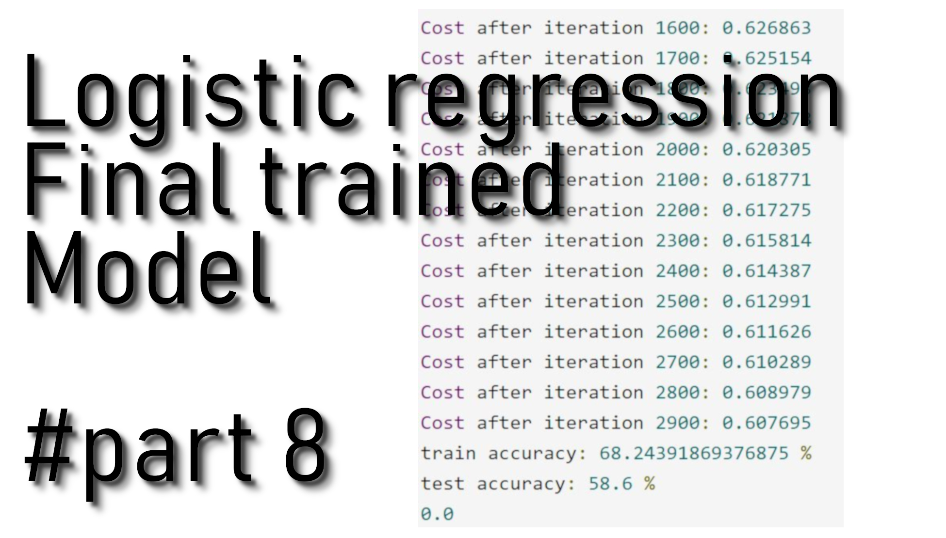
print(np.squeeze(my_predicted_image))

Bellow is our training results, as we did 3000 training steps, and as a result, we received test accuracy of 58.6% and train accuracy of 68.24%. This is not that accurate, but evaluating that we are using simple logistic regression, it's not that bad, even it predicted our image as a CAT!

Cost after iteration 100: 0.671626
Cost after iteration 200: 0.663768
Cost after iteration 300: 0.658534
Cost after iteration 400: 0.654486
Cost after iteration 500: 0.651100
Cost after iteration 600: 0.648129
Cost after iteration 700: 0.645438
Cost after iteration 800: 0.642949
Cost after iteration 900: 0.640613
Cost after iteration 1000: 0.638401
Cost after iteration 1100: 0.636290
Cost after iteration 1200: 0.634267
Cost after iteration 1300: 0.632320
Cost after iteration 1400: 0.630441
Cost after iteration 1500: 0.628624
Cost after iteration 1600: 0.626863
Cost after iteration 1700: 0.625154
Cost after iteration 1800: 0.623493
Cost after iteration 1900: 0.621878
Cost after iteration 2000: 0.620305
Cost after iteration 2100: 0.618771
Cost after iteration 2200: 0.617275
Cost after iteration 2300: 0.615814
Cost after iteration 2400: 0.614387
Cost after iteration 2500: 0.612991
Cost after iteration 2600: 0.611626
Cost after iteration 2700: 0.610289
Cost after iteration 2800: 0.608979
Cost after iteration 2900: 0.607695
train accuracy: 68.24391869376875 %
test accuracy: 58.6 %
0.0

Full tutorial code:

import os
import cv2
import numpy as np
import matplotlib.pyplot as plt
import scipy

ROWS = 64
COLS = 64
CHANNELS = 3

TRAIN_DIR = 'Train_data/'
TEST_DIR = 'Test_data/'

train_images = [TRAIN_DIR+i for i in os.listdir(TRAIN_DIR)]
test_images =  [TEST_DIR+i for i in os.listdir(TEST_DIR)]

def read_image(file_path):
    img = cv2.imread(file_path, cv2.IMREAD_COLOR)
    return cv2.resize(img, (ROWS, COLS), interpolation=cv2.INTER_CUBIC)

def prepare_data(images):
    m = len(images)
    X = np.zeros((m, ROWS, COLS, CHANNELS), dtype=np.uint8)
    y = np.zeros((1, m))
    for i, image_file in enumerate(images):
        X[i,:] = read_image(image_file)
        if 'dog' in image_file.lower():
            y[0, i] = 1
        elif 'cat' in image_file.lower():
            y[0, i] = 0
    return X, y

def sigmoid(z):
    s = 1/(1+np.exp(-z))
    return s

def propagate(w, b, X, Y):
    m = X.shape[1]
    
     # FORWARD PROPAGATION (FROM X TO COST)
    z = np.dot(w.T, X)+b # tag 1
    A = sigmoid(z) # tag 2                                    
    cost = (-np.sum(Y*np.log(A)+(1-Y)*np.log(1-A)))/m # tag 5
    
    # BACKWARD PROPAGATION (TO FIND GRAD)
    dw = (np.dot(X,(A-Y).T))/m # tag 6
    db = np.average(A-Y) # tag 7

    cost = np.squeeze(cost)
    grads = {"dw": dw,
             "db": db}
    
    return grads, cost

def optimize(w, b, X, Y, num_iterations, learning_rate, print_cost = False):
    costs = []    
    for i in range(num_iterations):
        # Cost and gradient calculation
        grads, cost = propagate(w, b, X, Y)
        
        # Retrieve derivatives from grads
        dw = grads["dw"]
        db = grads["db"]

        # update w and b
        w = w - learning_rate*dw
        b = b - learning_rate*db

        # Record the costs
        if i % 100 == 0:
            costs.append(cost)
            
        # Print the cost every 100 training iterations
        if print_cost and i % 100 == 0:
            print ("Cost after iteration %i: %f" %(i, cost))

    # update w and b to dictionary
    params = {"w": w,
              "b": b}
    
    # update derivatives to dictionary
    grads = {"dw": dw,
             "db": db}
    
    return params, grads, costs

def predict(w, b, X):    
    m = X.shape[1]
    Y_prediction = np.zeros((1, m))
    w = w.reshape(X.shape[0], 1)
    
    z = np.dot(w.T, X) + b
    A = sigmoid(z)
    
    for i in range(A.shape[1]):
        # Convert probabilities A[0,i] to actual predictions p[0,i]
        if A[0,i] > 0.5:
            Y_prediction[[0],[i]] = 1
        else: 
            Y_prediction[[0],[i]] = 0
    
    return Y_prediction

def initialize_with_zeros(dim):
    w = np.zeros((dim, 1))
    b = 0
    return w, b

def model(X_train, Y_train, X_test, Y_test, num_iterations = 2000, learning_rate = 0.5, print_cost = False):
	# initialize parameters with zeros
    w, b = initialize_with_zeros(X_train.shape[0])

    # Gradient descent
    parameters, grads, costs = optimize(w, b, X_train, Y_train, num_iterations, learning_rate, print_cost)
    
    # Retrieve parameters w and b from dictionary "parameters"
    w = parameters["w"]
    b = parameters["b"]
    
    # Predict test/train set examples
    Y_prediction_test = predict(w,b,X_test)
    Y_prediction_train = predict(w,b,X_train)

    # Print train/test Errors
    print("train accuracy: {} %".format(100 - np.mean(np.abs(Y_prediction_train - Y_train)) * 100))
    print("test accuracy: {} %".format(100 - np.mean(np.abs(Y_prediction_test - Y_test)) * 100))

    
    dict = {"costs": costs,
            "Y_prediction_test": Y_prediction_test,
            "Y_prediction_train": Y_prediction_train,
            "w": w,
            "b": b,
            "learning_rate": learning_rate,
            "num_iterations:": num_iterations}
    
    return dict

train_set_x, train_set_y = prepare_data(train_images)
test_set_x, test_set_y = prepare_data(test_images)

train_set_x_flatten = train_set_x.reshape(train_set_x.shape[0], ROWS*COLS*CHANNELS).T
test_set_x_flatten = test_set_x.reshape(test_set_x.shape[0], -1).T

train_set_x = train_set_x_flatten/255
test_set_x = test_set_x_flatten/255

d = model(train_set_x, train_set_y, test_set_x, test_set_y, num_iterations = 3000, learning_rate = 0.003, print_cost = True)

test_image = "cat.jpg"
my_image = read_image(test_image).reshape(1, ROWS*COLS*CHANNELS).T
my_predicted_image = predict(d["w"], d["b"], my_image)
print(np.squeeze(my_predicted_image))