This tutorial will guide you through the simplest way to download historical cryptocurrency OHCL market data via exchange APIs. We'll use this data to train our Reinforcement Learning Bitcoin trading agent that could finally beat the market!

Algorithmic trading is a popular way to address the rapidly changing and volatile environment of cryptocurrency markets. However, implementing an automated trading strategy is challenging and requires a lot of backtesting, which involves a lot of historical data and computational power. While developing a Bitcoin RL trading bot, I found out that it's pretty hard to get lower timeframe historical timeframe data. While there are many sources on the market that offer historical cryptocurrency data, most of them have drawbacks. Many of them are required to pay for such data and are not that cheap. Sources for free data provide only insufficient temporal resolution data (daily) or cover limited periods of a limited amount of currency pairs. This tutorial will show you that obtaining historical open, high, low, close data (OHLC) at a 1-minute or whatever resolution you need is not a magical task that could be done in a few lines of Python code without spending any money.

Installing the API

This tutorial will show you how to use the Bitfinex exchange API to download historical OHCL data. However, this approach also works for any other exchange that provides a similar API, but I chose Bitfinex right now. Also, if you don't have a Bitfinex account, don't worry. This can be done without it because we will only use public API endpoints. If you are not familiar with what an API is, how it works or how to use it, you can read about it on the Bitfinex API documentation. This is also the interface through which our algorithm will interact with the exchange. But don't worry, there are already several implementations available; we won't need to write the Python interface for communication. For this, I'll use bitfinex-tencars, the python library, which can be installed via pip: pip install bitfinex-tencars

It's pretty old, but it doesn't matter while it works for us. Also, we could use another library like the bitfinex-api-py, which allows us to make live trades. Still, because this tutorial is not about live Python trading, I'd better use the bitfinex-tencars package.

Using the API client

Looking at the Bitfinex API documentation, we would see two API versions, v1 and v2, both implemented in the client we just installed, but I chose only to use the v2 API. After importing the Bitfinex API client python library, we need to create an instance of the v2 API by running the code below. Please pay attention that we are not providing any keys here, so we will only have access to the public endpoints. This means that there are no ways to risk somehow losing our balance in the Bitfinex account. Of course, the corresponding message will be shown after we'll run the code.

import bitfinex
# Create api instance of the v2 API
api_v2 = bitfinex.bitfinex_v2.api_v2()

And that is how we open gates to our historical market data. From the Bitfinex documentation, we saw that one of the public endpoints is called candles, which returns the data behind the candlestick charts on all the exchanges. This kind of data contains a timestamp, open, close, high and low price, and usually the trade volume. At first, we will try the simplest way to interact with this endpoint through the client by just calling it with its default settings.

result = api_v2.candles()
print(len(result))

The line above will give us the last 1000 minutes of OHLC data for the BTC/USD price. That's a nice achievement, but we usually are interested in a period long ago or different currency pairs. To achieve specifically what we want, we should specify the following parameters:

• symbol: currency pair,default: BTCUSD;
• interval: temporal resolution, e.g., 1m for 1 minute of OHLC data;
• limit: number of returned data points, default: 1000;
• start: start time of interval in milliseconds since 1970;
• end: end time of interval in milliseconds since 1970.

Now we can write and run our first query. The code below will return the 1-hour resolution OHLC data of BTC/USD for the first month in September 2020.

import bitfinex
import datetime
import time
import pandas as pd

# Create api instance of the v2 API
api_v2 = bitfinex.bitfinex_v2.api_v2()

# Define query parameters
pair = 'BTCUSD' # Currency pair of interest
TIMEFRAME = '1h'#,'4h','1h','15m','1m'

# Define the start date
t_start = datetime.datetime(2018, 9, 1, 0, 0)
t_start = time.mktime(t_start.timetuple()) * 1000

# Define the end date
t_stop = datetime.datetime(2020, 10, 1, 0, 0)
t_stop = time.mktime(t_stop.timetuple()) * 1000

# Download OHCL data from API
result = api_v2.candles(symbol=pair, interval=TIMEFRAME, limit=1000, start=t_start, end=t_stop)

# Convert list of data to pandas dataframe
names = ['Date', 'Open', 'Close', 'High', 'Low', 'Volume']
df = pd.DataFrame(result, columns=names)
df['Date'] = pd.to_datetime(df['Date'], unit='ms')

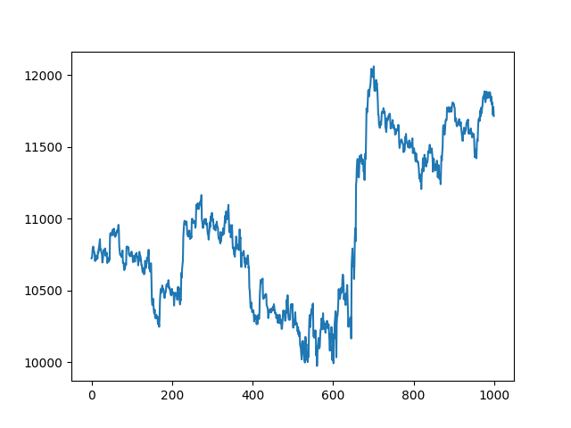
# we can plot our downloaded data
import matplotlib.pyplot as plt
plt.plot(df['Open'],'-')
plt.show()

At the end of the above script, I added a few Matplotlib lines so that we could plot our downloaded data, which looks following:

Historical data for a longer time interval

So, now we know how to download 1000 historical data steps, but how to download more data if API can't download more data at once. So if we were to increase the time interval of interest to the entire year, for example, we would not be able to get it at a 1-hour resolution. So to get past this limitation, we need to write a function that would split our big query into multiple minor queries. Also, I must mention that we need to keep in mind that there is a limit to how many requests we can make to the Bitfinex API. Currently, this limit is 60 calls per minute, which means that after each request, we should wait for a minimum of 1 second before we start the next call. The function below remains 1.5 seconds to be safe, but you can change that if you want.

def fetch_data(start, stop, symbol, interval, TIMEFRAME_S):
    limit = 1000    # We want the maximum of 1000 data points
    # Create api instance
    api_v2 = bitfinex.bitfinex_v2.api_v2()
    hour = TIMEFRAME_S * 1000
    step = hour * limit
    data = []

    total_steps = (stop-start)/hour
    while total_steps > 0:
        if total_steps < limit: # recalculating ending steps
            step = total_steps * hour

        end = start + step
        data += api_v2.candles(symbol=symbol, interval=interval, limit=limit, start=start, end=end)
        print(pd.to_datetime(start, unit='ms'), pd.to_datetime(end, unit='ms'), "steps left:", total_steps)
        start = start + step
        total_steps -= limit
        time.sleep(1.5)
    return data

With the function above, now we can run queries for longer time intervals. The only extra thing we need to calculate and provide is the step size in milliseconds. We recalculate the step size every new while loop to know how many data points we should ask in every new minor query. This is very similar to the limit we defined before. To reduce the number of requests we do to the API, it would be best to go for the maximum step size. For the 1-minute case, the one-step size is calculated following:

time = seconds * limit * 1000ms
1-min = 60s * 1000 * 1000 = 60000000
1hour = 3600s * 1000 * 1000 = 3600000000

Finally, we want to convert the results into a Pandas data frame. Then we can remove potential duplicates, make sure that everything is in the correct order, and restore the numerical timestamp into a human-readable format. In the final step, we can save our downloaded historical data and save it to a .csv file:

result = fetch_data(t_start, t_stop, pair, TIMEFRAME, TIMEFRAME_S)
names = ['Date', 'Open', 'Close', 'High', 'Low', 'Volume']
df = pd.DataFrame(result, columns=names)
df.drop_duplicates(inplace=True)
df['Date'] = pd.to_datetime(df['Date'], unit='ms')
df.set_index('Date', inplace=True)
df.sort_index(inplace=True)
df.to_csv(f"{pair}_{TIMEFRAME}.csv")

Here is the complete code to download long historical data:

import bitfinex
import datetime
import time
import pandas as pd

# Define query parameters
pair = 'BTCUSD' # Currency pair of interest
TIMEFRAME = '1h'#,'4h','1h','15m','1m'
TIMEFRAME_S = 3600 # seconds in TIMEFRAME

# Define the start date
t_start = datetime.datetime(2018, 1, 1, 0, 0)
t_start = time.mktime(t_start.timetuple()) * 1000

# Define the end date
t_stop = datetime.datetime(2020, 10, 12, 0, 0)
t_stop = time.mktime(t_stop.timetuple()) * 1000

def fetch_data(start, stop, symbol, interval, TIMEFRAME_S):
    limit = 1000    # We want the maximum of 1000 data points
    # Create api instance
    api_v2 = bitfinex.bitfinex_v2.api_v2()
    hour = TIMEFRAME_S * 1000
    step = hour * limit
    data = []

    total_steps = (stop-start)/hour
    while total_steps > 0:
        if total_steps < limit: # recalculating ending steps
            step = total_steps * hour

        end = start + step
        data += api_v2.candles(symbol=symbol, interval=interval, limit=limit, start=start, end=end)
        print(pd.to_datetime(start, unit='ms'), pd.to_datetime(end, unit='ms'), "steps left:", total_steps)
        start = start + step
        total_steps -= limit
        time.sleep(1.5)
    return data

result = fetch_data(t_start, t_stop, pair, TIMEFRAME, TIMEFRAME_S)
names = ['Date', 'Open', 'Close', 'High', 'Low', 'Volume']
df = pd.DataFrame(result, columns=names)
df.drop_duplicates(inplace=True)
df['Date'] = pd.to_datetime(df['Date'], unit='ms')
df.set_index('Date', inplace=True)
df.sort_index(inplace=True)
df.to_csv(f"{pair}_{TIMEFRAME}.csv")

If you wonder how many currency pairs of historical data you can download through the Bitfinex API, just run the two following code lines:

api_v1 = bitfinex.bitfinex_v1.api_v1()
pairs = api_v1.symbols()

Train our model on multiple environments

One of the significant problems we face with the current RL Bitcoin trading bot is that it takes too long to train it to see some satisfying results. I am using quite a low learning rate (lr=0.00001), we could train it much faster while using a bigger one, but then our model may not learn important price action features. So, it's pretty evident that, in some kind, we should speed up our learning process. One of the best ways that come to my head is that we should use multiprocessing. If you were following my past tutorials, you should already be familiar with my BipedalWalker-v3 Reinforcement learning tutorial, where I used multiple environments to train my agent. I tested that we were not winning a lot of speed while running multiple environments in the background and detecting states for each environment. So, we created 16 running environments, and we detected their next state in a batch - this is how to speed it up.

In this part, I decided that I needed to do similar stuff. We'll reconstruct our custom environment so that we can start multiple of them in the background. This way, our bot will have the opportunity to try more different trade combinations and learn price action features faster.

Multiprocessing example

While we talk about python multiprocessing, I am not a pro, but I have successfully implemented it in several past projects. First, I'll show you a simple example where we'll use pipe communication between multiple processes. Then I'll show you how I similarly implemented our custom environment.

First of all, I am not going to explain step-by-step how python multiprocessing works. I'll discuss the concept of data sharing and message passing between custom environment processes while using the multiprocessing module.

In our case, any newly created processed environment will do the following:

• run independently;
• have their own memory space.

Below you can see my example code to understand the basics of multiprocessing. So I created a class called class Environment(Process) that will start an independent process running in the background.

For simplicity, my processes, as a result, will return the received number multiplied by 2.

For simplicity, I create only two custom processes within this custom environment. For communication between the main program and environment, processes will use a pipe communication method. Pipe() returns two connection objects which represent the two ends of the pipe. Each connection object has send() and recv() methods.

from multiprocessing import Process, Pipe
import time
import random

class Environment(Process): # creating environment class for multiprocessing
    def __init__(self, env_idx, child_conn):
        super(Environment, self).__init__()
        self.env_idx = env_idx
        self.child_conn = child_conn

    def run(self):
        super(Environment, self).run()
        while True:
            number = self.child_conn.recv()
            self.child_conn.send(number*2)

if __name__ == "__main__":
    works, parent_conns, child_conns = [], [], []
    
    for idx in range(2):
        parent_conn, child_conn = Pipe() # creating a communication pipe
        work = Environment(idx, child_conn) # creating new process 
        work.start() # starting process 
        works.append(work) # saving started procsses to list
        parent_conns.append(parent_conn) # saving communication pipe refference to list
        child_conns.append(child_conn) # saving communication pipe refference to list

    while True:
        for worker_id, parent_conn in enumerate(parent_conns):
            r = random.randint(0, 10) # creating random number between 0 and 10
            parent_conn.send(r) # sending message with random nuber to worker_id running process
            
        time.sleep(1)

        for worker_id, parent_conn in enumerate(parent_conns):
            result = parent_conn.recv() # reading received message from worker_id process
            print(f"From {worker_id} worker received {result}")

This is quite simple code. In the main loop, I generate a random number for each process between 0 and 10 and send it. Not to spam my console, I use 1-second sleep, and then I run another loop to read pipe for answers and print it to our screen.

Multiprocessing environment

In a similar principle works our multiprocessing environment with a custom Bitcoin trading bot. Instead of giving us back a simple number, we'll run our custom trading environment to make a predicted action and return a state, reward, and other parameters of a particular environment.

Of course, it's much easier to tell than to convert my words to code because while programming a script to work with multiple processes, sometimes it's pretty complicated to debug. But lucky you, I already did this tricky job for you, so simply, here is code that we'll use to create independent environments running in the background:

from multiprocessing import Process, Pipe

class Environment(Process):
    def __init__(self, env_idx, child_conn, env, training_batch_size, visualize):
        super(Environment, self).__init__()
        self.env = env
        self.env_idx = env_idx
        self.child_conn = child_conn
        self.training_batch_size = training_batch_size
        self.visualize = visualize

    def run(self):
        super(Environment, self).run()
        state = self.env.reset(env_steps_size = self.training_batch_size)
        self.child_conn.send(state)
        while True:
            reset, net_worth, episode_orders = 0, 0, 0
            action = self.child_conn.recv()
            if self.env_idx == 0:
                self.env.render(self.visualize)
            state, reward, done = self.env.step(action)

            if done or self.env.current_step == self.env.end_step:
                net_worth = self.env.net_worth
                episode_orders = self.env.episode_orders
                state = self.env.reset(env_steps_size = self.training_batch_size)
                reset = 1

            self.child_conn.send([state, reward, done, reset, net_worth, episode_orders])

This environment returns [state, reward, done, reset, net_worth, episode_orders] parameters, which will help us track each environment's statistics and make proper action predictions.

Multiprocessing training agents

This part is quite complicated, and I think I'm not committed to explaining its code. So I'll give you a function that we'll use every time we train our custom Bitcoin Reinforcement Learning trading agent. All the network parameters are defined in the same way as before. Apart from that, now we can set how many workers we want to create with the num_worker parameter. Before choosing the correct number of your workers, consider what CPU and GPU you have. You can run more workers if you have GPU because training will be done on a graphical processing unit, and environments will run on a process. Otherway, if you don't have GPU, you won't get significant speed improvement because the hardest part (training) will be done on the CPU. Anyway, here is the code:

def train_multiprocessing(CustomEnv, agent, train_df, num_worker=4, training_batch_size=500, visualize=False, EPISODES=10000):
    works, parent_conns, child_conns = [], [], []
    episode = 0
    total_average = deque(maxlen=100) # save recent 100 episodes net worth
    best_average = 0 # used to track best average net worth

    for idx in range(num_worker):
        parent_conn, child_conn = Pipe()
        env = CustomEnv(train_df, lookback_window_size=agent.lookback_window_size)
        work = Environment(idx, child_conn, env, training_batch_size, visualize)
        work.start()
        works.append(work)
        parent_conns.append(parent_conn)
        child_conns.append(child_conn)

    agent.create_writer(env.initial_balance, env.normalize_value, EPISODES) # create TensorBoard writer

    states =        [[] for _ in range(num_worker)]
    next_states =   [[] for _ in range(num_worker)]
    actions =       [[] for _ in range(num_worker)]
    rewards =       [[] for _ in range(num_worker)]
    dones =         [[] for _ in range(num_worker)]
    predictions =   [[] for _ in range(num_worker)]

    state = [0 for _ in range(num_worker)]
    for worker_id, parent_conn in enumerate(parent_conns):
        state[worker_id] = parent_conn.recv()

    while episode < EPISODES:
        predictions_list = agent.Actor.actor_predict(np.reshape(state, [num_worker]+[_ for _ in state[0].shape]))
        actions_list = [np.random.choice(agent.action_space, p=i) for i in predictions_list]

        for worker_id, parent_conn in enumerate(parent_conns):
            parent_conn.send(actions_list[worker_id])
            action_onehot = np.zeros(agent.action_space.shape[0])
            action_onehot[actions_list[worker_id]] = 1
            actions[worker_id].append(action_onehot)
            predictions[worker_id].append(predictions_list[worker_id])

        for worker_id, parent_conn in enumerate(parent_conns):
            next_state, reward, done, reset, net_worth, episode_orders = parent_conn.recv()
            states[worker_id].append(np.expand_dims(state[worker_id], axis=0))
            next_states[worker_id].append(np.expand_dims(next_state, axis=0))
            rewards[worker_id].append(reward)
            dones[worker_id].append(done)
            state[worker_id] = next_state

            if reset:
                episode += 1
                a_loss, c_loss = agent.replay(states[worker_id], actions[worker_id], rewards[worker_id], predictions[worker_id], dones[worker_id], next_states[worker_id])
                total_average.append(net_worth)
                average = np.average(total_average)

                agent.writer.add_scalar('Data/average net_worth', average, episode)
                agent.writer.add_scalar('Data/episode_orders', episode_orders, episode)
                
                print("episode: {:<5} worker: {:<1} net worth: {:<7.2f} average: {:<7.2f} orders: {}".format(episode, worker_id, net_worth, average, episode_orders))
                if episode > len(total_average):
                    if best_average < average:
                        best_average = average
                        print("Saving model")
                        agent.save(score="{:.2f}".format(best_average), args=[episode, average, episode_orders, a_loss, c_loss])
                    agent.save()
                
                states[worker_id] = []
                next_states[worker_id] = []
                actions[worker_id] = []
                rewards[worker_id] = []
                dones[worker_id] = []
                predictions[worker_id] = []

    agent.end_training_log()
    # terminating processes after while loop
    works.append(work)
    for work in works:
        work.terminate()
        print('TERMINATED:', work)
        work.join()

Ok, probably you need an example of how to use this above function, right? It's not that different as it was before; here is an example of how I trained the Dense RL network:

from multiprocessing_env import train_multiprocessing, test_multiprocessing
...

if __name__ == "__main__":            
    df = pd.read_csv('./BTCUSD_1h.csv')
    df = df.sort_values('Date')
    df = AddIndicators(df) # insert indicators to df

    lookback_window_size = 50
    test_window = 720*3 # 3 months 
    train_df = df[100:-test_window-lookback_window_size] # we leave 100 to have properly calculated indicators
    test_df = df[-test_window-lookback_window_size:]
    
    agent = CustomAgent(lookback_window_size=lookback_window_size, lr=0.00001, epochs=5, optimizer=Adam, batch_size = 32, model="Dense")
    train_multiprocessing(CustomEnv, agent, train_df, num_worker = 32, training_batch_size=500, visualize=False, EPISODES=200000)

The main parameters you can change are the following: lookback_window_size, learning rate (lr), epochs, optimizer, batch_size, model type, workers count, training_batch_size, training episodes.

Suppose you think this is a lot of parameters; here, I give only the most critical parameters. In that case, much more might be changed when we start talking about optimizing our model, but from training and testing results, you'll see that it's enough parameters to create a primary view of a model.

If you watched my previous tutorial, you already should know that I created three different models (Dence, CNN, and LSTM). So I trained all 3 of them, and I can show you my training results and parameters for each model in the following table:

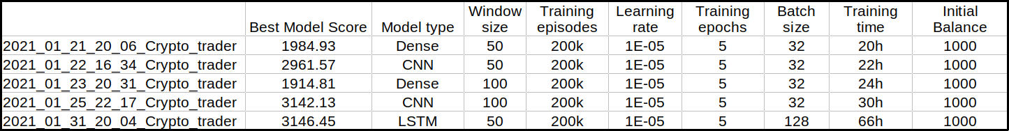
As you can see, I mostly tried to change model type, windows size, and batch size. As a result, I looked to "Best Model Score" and training time. You can decide which model is best from this data, and I lean towards the CNN network. Of course, LSTM is also quite impressive, but it requires more than two times longer to train.

Below is a snip from Tensorboard:

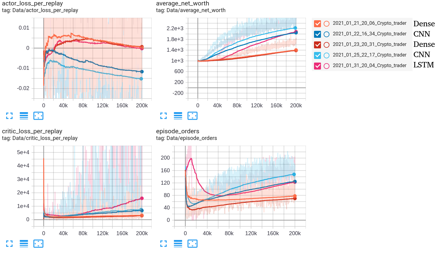
First, I will give you a short explanation about loss curves:

• Actor Loss - is the average size of the Actor loss function. Correlates to how much the policy (process for deciding actions) is changing. This should decrease during a successful training session. These values will fluctuate during the training. Generally, they should be less than 1.0;
• Critic Loss - is the average size of the Critic loss function. Correlates to how well the Critic model can predict the value of each state. Critic loss will increase as the reward increases, and when the reward becomes stable, the loss should decrease. This should increase while the agent is learning, and as the reward stabilizes, it should fall.

From the above training results, it's pretty hard to guess what model will be the best with validation data, but we can assume it should have the best model score. So it should be CNN or LSTM network. We'll find out after testing both of them.

Multiprocessing testing agents

No less important is the testing phase for us, so I also wrote a multiprocessing script to test our trained models:

def test_multiprocessing(CustomEnv, agent, test_df, num_worker = 4, visualize=False, test_episodes=1000, folder="", name="Crypto_trader", comment="", initial_balance=1000):
    agent.load(folder, name)
    works, parent_conns, child_conns = [], [], []
    average_net_worth = 0
    average_orders = 0
    no_profit_episodes = 0
    episode = 0

    for idx in range(num_worker):
        parent_conn, child_conn = Pipe()
        env = CustomEnv(test_df, initial_balance=initial_balance, lookback_window_size=agent.lookback_window_size)
        work = Environment(idx, child_conn, env, training_batch_size=0, visualize=visualize)
        work.start()
        works.append(work)
        parent_conns.append(parent_conn)
        child_conns.append(child_conn)

    state = [0 for _ in range(num_worker)]
    for worker_id, parent_conn in enumerate(parent_conns):
        state[worker_id] = parent_conn.recv()

    while episode < test_episodes:
        predictions_list = agent.Actor.actor_predict(np.reshape(state, [num_worker]+[_ for _ in state[0].shape]))
        actions_list = [np.random.choice(agent.action_space, p=i) for i in predictions_list]

        for worker_id, parent_conn in enumerate(parent_conns):
            parent_conn.send(actions_list[worker_id])

        for worker_id, parent_conn in enumerate(parent_conns):
            next_state, reward, done, reset, net_worth, episode_orders = parent_conn.recv()
            state[worker_id] = next_state

            if reset:
                episode += 1
                #print(episode, net_worth, episode_orders)
                average_net_worth += net_worth
                average_orders += episode_orders
                if net_worth < initial_balance: no_profit_episodes += 1 # calculate episode count where we had negative profit through episode
                print("episode: {:<5} worker: {:<1} net worth: {:<7.2f} average_net_worth: {:<7.2f} orders: {}".format(episode, worker_id, net_worth, average_net_worth/episode, episode_orders))
                if episode == test_episodes: break
            
    print("No profit episodes: {}".format(no_profit_episodes))
    # save test results to test_results.txt file
    with open("test_results.txt", "a+") as results:
        current_date = datetime.now().strftime('%Y-%m-%d %H:%M')
        results.write(f'{current_date}, {name}, test episodes:{test_episodes}')
        results.write(f', net worth:{average_net_worth/(episode+1)}, orders per episode:{average_orders/test_episodes}')
        results.write(f', no profit episodes:{no_profit_episodes}, comment: {comment}\n')
    
    # terminating processes after while loop
    works.append(work)
    for work in works:
        work.terminate()
        print('TERMINATED:', work)
        work.join()

Ok, probably the same as with the training part; you need an example of using this above function, right? It's not that different as it was before; here is an example of how I trained the Dense RL network:

from multiprocessing_env import train_multiprocessing, test_multiprocessing
...

if __name__ == "__main__":            
    df = pd.read_csv('./BTCUSD_1h.csv')
    df = df.sort_values('Date')
    df = AddIndicators(df) # insert indicators to df

    lookback_window_size = 50
    test_window = 720*3 # 3 months 
    train_df = df[100:-test_window-lookback_window_size] # we leave 100 to have properly calculated indicators
    test_df = df[-test_window-lookback_window_size:]
    
    agent = CustomAgent(lookback_window_size=lookback_window_size, lr=0.00001, epochs=5, optimizer=Adam, batch_size = 32, model="Dense")
    test_multiprocessing(CustomEnv, agent, test_df, num_worker = 16, visualize=False, test_episodes=1000, folder="2021_01_21_20_06_Crypto_trader", name="1984.93_Crypto_trader", comment="Dense")

Usually, we call test_multiprocessing on our test_df dataset, set episodes testing count, give a path to our trained model, and that's it. Testing is a much less resource-hungry process, so testing all my trained models is not a problem. Results are in the following table:

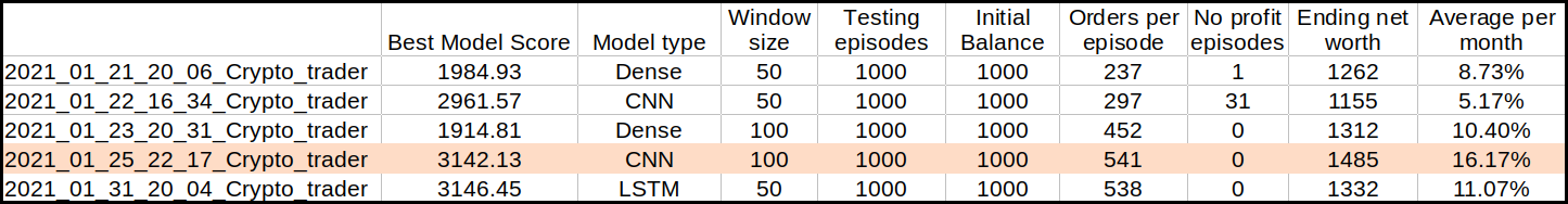
I must note that these results are for unseen data! In my previous tutorial, the most critical parameters are "No profit episodes" and "Ending net worth". Looking at them, we can evaluate how good our model is. I highlighted the (CNN) model with the highest ending net worth on our testing dataset in the above table. In 3 months, this agent grew our net worth by 48%, and if we average this number to each month, that's around 16.17%, impressive! In the previous tutorial, we saw that CNN wasn't performing that well, but I thought that this might be because of short training data. My theory was confirmed; we needed more training data.

Conclusion:

So retrieving high-resolution OHLC data is not that complicated. It's much easier to use Python script and download it than google it for hours, where you can download it for free.

So, I proved that actually, it's possible to beat the market with Neural Networks. However, I am still skeptical about running it for live trading; I do not recommend it to you. There is still a lot of stuff where this bot could be improved.

So far, trades in our simulation are taking place on perfect terms, so we'll add fees to all trades we do in the next tutorial. Also, maybe we'll add much more indicators, that our model could learn more market features. Also, I think my data normalization technique is not the best. I hope to do some investigation into this part.

Thanks for reading! As always, all the code given in this tutorial can be found on my GitHub page and is free to use!

All of these tutorials are for educational purposes and should not be taken as trading advice. It would be best to not trade based on any algorithms or strategies defined in this, previous, or future tutorials, as you are likely to lose your investment.