In this tutorial, we will continue developing a Bitcoin trading bot. We'll integrate more technical indicators into our code, we try a newly proposed normalization technique, and of course, I'll slightly modify the whole code that it could be much easier to test our trained models.

Welcome back to my 7th tutorial part with the Reinforcement Learning Bitcoin trading bot. To get to where we are now, I wrote thousands of code lines and spent thousands of hours training my models. But if someone told me that getting to the current 7th tutorial would have cost me so much, I am not sure if I would be starting doing this tutorial series.

On the other hand, I'm proud that I didn't give up, and no matter how hard it was or didn't know the solutions from a particular moment, I tried to find the strength to move forward with my projects. This is called self-motivation, and I did this not for myself but for everyone who will read my tutorial series.

Looking at what we have done so far, I can't believe it by myself. We created a Bitcoin trading bot that could beat the market in our simulation! So far, we have created a Reinforcement Learning cryptocurrency trading environment where we can simulate our trades by using multiprocessing to speed everything up. Also, we found an easy way to download Historical marked data. We tested several (CNN, LSTM, Dense) Neural Networks architectures to measure their performance. All this is only a tiny part of what we have done!

So far, trades in our simulation were taking place on perfect terms. So in this tutorial part, I decided to insert order fees into our model, add more uncorrelated indicators, implement a solution to normalize our training/testing data, and implement a solution to test our different models without remembering training settings. So this part might be one of the most interesting and exciting!

Normalizing Data

Until this moment, I didn't use any normalization techniques. I divided all values by 40k. But I want to point out that time-series data is not stationary (you can google what it means). This means that it's hard for a machine learning model to predict a downtrend if it was learned on uptrend data while training.

We can solve this by using differencing and transformation techniques to convert our data to a more normal distribution form.

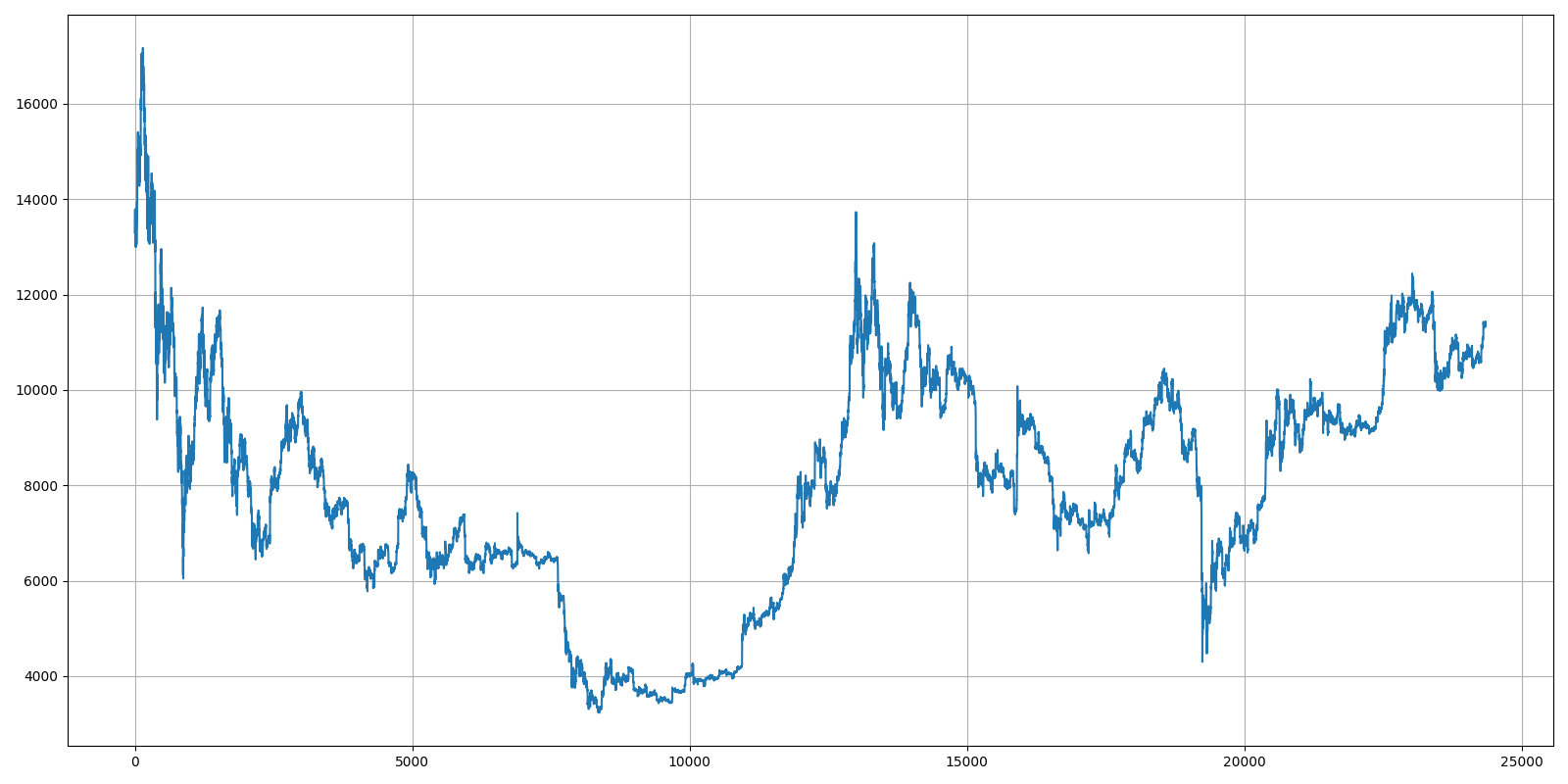
This is how our market data looks like if we'll plot only Close price:

Differencing is a process where we subtract the derivative (rate of return) at each time step from the value at a previous time step. We do this with one simple line: df["Close"] = df["Close"] - df["Close"].shift(1)

As a result, this should remove a trend and receive the following results:

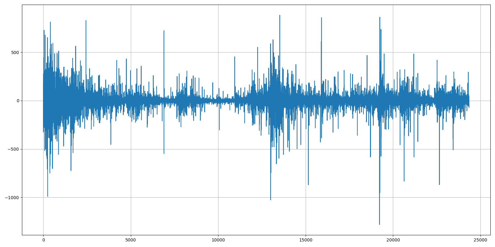
Results look pretty interesting, and it seems that the visual trend was removed. However, the data still has a clear seasonality. We can try to remove that by taking the logarithm at every time step before differencing our data. It's very similar to the above line: df["Close"] = np.log(df["Close"]) - np.log(df["Close"].shift(1))

Now we receive the following chart:

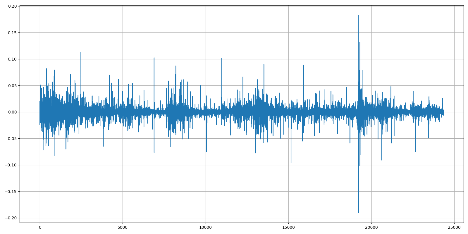
Now it's evident that we humans can't tell that our Bitcoin historical data is in this chart. In the last step, we'll take this data and normalize this data by putting it between 0 and 1:

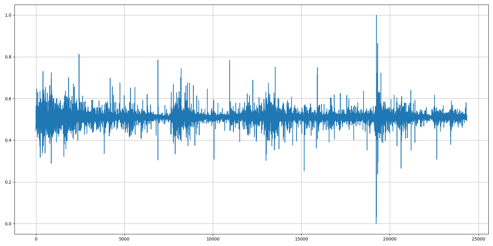
And there are a few lines of code I used to receive all four above plots:

if __name__ == "__main__":
    # testing normalization technieques
    df = pd.read_csv('./BTCUSD_1h.csv')
    df = df.dropna()
    df = df.sort_values('Date')

    #df["Close"] = df["Close"] - df["Close"].shift(1)
    df["Close"] = np.log(df["Close"]) - np.log(df["Close"].shift(1))

    Min = df["Close"].min()
    Max = df["Close"].max()
    df["Close"] = (df["Close"] - Min) / (Max - Min)
    
    fig = plt.figure(figsize=(16,8)) 
    plt.plot(df["Close"],'-')
    ax=plt.gca()
    ax.grid(True)
    fig.tight_layout()
    plt.show()

Technical Indicators

In my 5th tutorial of this series, I showed you how to insert indicators into our market data. At that tutorial, I inserted five indicators: SMA, Bollinger Bands, Parabolic SAR, MACD, and RSI. Also, at the end of that tutorial, I mentioned that we'd try to insert more of them later, and I think this tutorial is an excellent time for this task.

Usually, technical indicators are used for some technical analysis. Still, we'll call this "Feature engineering" because we'll try to extract only the most minor correlated indicators from a batch. We'll normalize them with the above-given technique, and everything will be fed to our Reinforcement Learning agent.

To choose the technical indicators that we'll use, we will compare the correlation of all 42 (at the moment of writing this tutorial) technical indicators in the ta library. The simplest way is to use pandas and seaborn libraries to find the correlation between each indicator of the same type (trend, volatility, volume, momentum, others). Then we'll select only the most minor correlated indicators of each kind. In my opinion, this way we can get as much benefit as possible, without adding too much noise to our state size.

Correlation and why it's important?

One of the fastest ways to enhance a machine learning model is to identify and reduce the highly correlated dataset features. These features add noise and inaccuracy to our model, making it harder to achieve the desired result.

When two independent features have a strong relationship, they are considered positively or negatively correlated. It's recommended to avoid highly correlated variables when developing models because they can skew the output. If two independent variables represent the same event, it can cause "noise" or inaccuracy in the model. The models rely only on external information to generate useful output, and having collinear (correlating) variables can increase variation in at least one of the regression outputs. This makes it challenging to understand which variable influences the dependent variable, making it difficult to assess the model's usefulness.

I am not going deep into explaining why, where, and how. There is plenty of information elsewhere. I'll keep on practical stuff.

First, I'll shortly explain the function that I use to drop correlated features and plot the visualization:

def DropCorrelatedFeatures(df, threshold, plot):
    df_copy = df.copy()

    # Remove OHCL columns
    df_drop = df_copy.drop(["Date", "Open", "High", "Low", "Close", "Volume"], axis=1)

    # Calculate Pierson correlation
    df_corr = df_drop.corr()

    columns = np.full((df_corr.shape[0],), True, dtype=bool)
    for i in range(df_corr.shape[0]):
        for j in range(i+1, df_corr.shape[0]):
            if df_corr.iloc[i,j] >= threshold or df_corr.iloc[i,j] <= -threshold:
                if columns[j]:
                    columns[j] = False
                    
    selected_columns = df_drop.columns[columns]

    df_dropped = df_drop[selected_columns]

    if plot:
        # Plot Heatmap Correlation
        fig = plt.figure(figsize=(8,8))
        ax = sns.heatmap(df_dropped.corr(), annot=True, square=True)
        ax.set_yticklabels(ax.get_yticklabels(), rotation=0) 
        ax.set_xticklabels(ax.get_xticklabels(), rotation=45, horizontalalignment='right')
        fig.tight_layout()
        plt.show()
    
    return df_dropped

As you can see, while reading the above function, first, I remove OHCL columns from my panda's data frame. It's not necessary to calculate the correlation for them. Next, calculating correlation is as simple as writing one line of code: df_corr = df_drop.corr(). That's it, and now we need to drop indicators that are above our threshold. There should be something similar and straightforward as calculating correlation, but I couldn't find that, so I used a for loop to do that. And lastly, I wrote code lines for beautiful heatmap visualization. This was done specifically for this tutorial. I'll use this function to plot the heatmap of each indicator type.

Trend indicators

The most significant part of fundamental indicators in ta library is trend indicators. In total, there are 14 given indicators. Trend indicators tell us which direction the market is moving in, of course, if there is a trend at all. I will not name each of these indicators, and this would be a waste of my and your time. So, below is a function that we will use to get a Heatmap of the trend indicators:

def get_trend_indicators(df, threshold=0.5, plot=False):
    df_trend = df.copy()
    
    # add custom trend indicators
    df_trend["sma7"] = SMAIndicator(close=df["Close"], window=7, fillna=True).sma_indicator()
    df_trend["sma25"] = SMAIndicator(close=df["Close"], window=25, fillna=True).sma_indicator()
    df_trend["sma99"] = SMAIndicator(close=df["Close"], window=99, fillna=True).sma_indicator()

    df_trend = add_trend_ta(df_trend, high="High", low="Low", close="Close")

    return DropCorrelatedFeatures(df_trend, threshold, plot)

As you can see, here I added 3 of my custom indicators, sma7, sma25, and sma99; similarly, you can add your indicators. So, probably you may be asking right now how to use this function, right? It can't be simpler; we do it following:

df = pd.read_csv('./BTCUSD_1h.csv')
df = df.sort_values('Date')
get_trend_indicators(df, threshold=0.5, plot=True)

I chose to use a threshold of 0.5 and a plot as True, just for visualization. By running the above code, we get the following heatmap as a result:

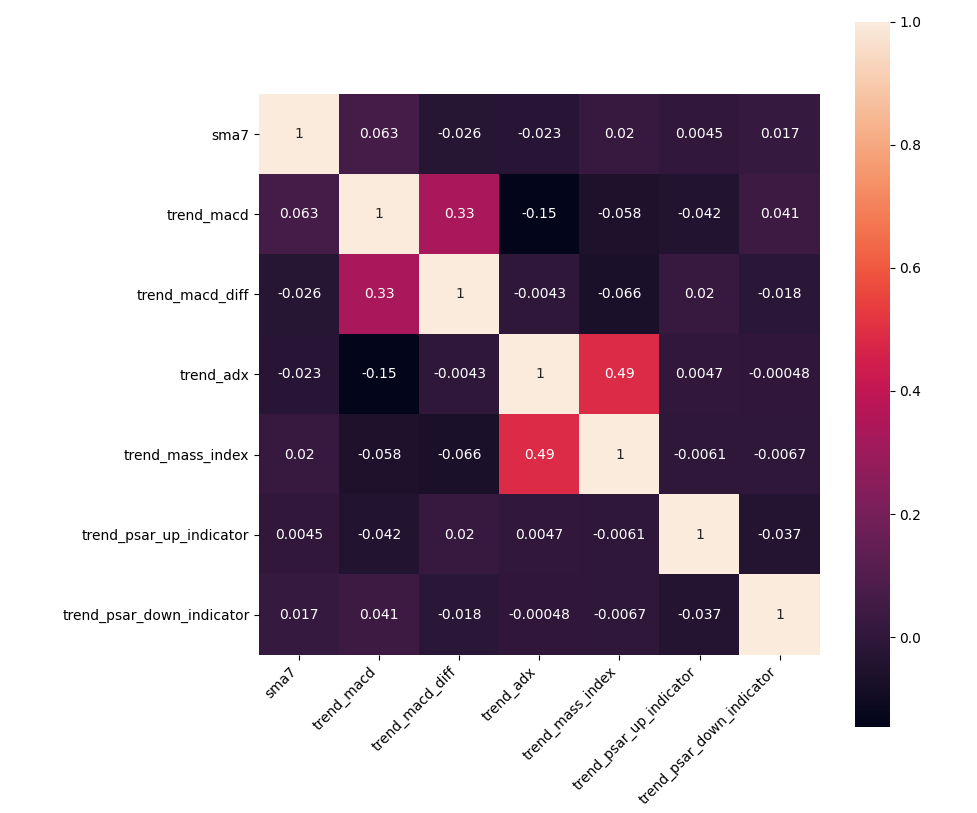
Before calculating the heatmap, there were 14+3 indicators. In total, this was 17 indicators; after dropping correlated ones, there left only 7 of them. This means that 59% of all trend indicators were correlating.

Volatility indicators

The second batch of indicators is five volatility indicators. That's a unique technical indicator that measures how far an asset strays from its mean directional value. This might sound complicated, but it is pretty simple: It strays far from its average direction when an asset has high volatility. For example, an earthquake has high volatility compared to expected weather conditions. Very similar to trend indicators, I created a function that we will use to get a Heatmap of the volatility indicators:

def get_volatility_indicators(df, threshold=0.5, plot=False):
    df_volatility = df.copy()
    
    # add custom volatility indicators
    # ...

    df_volatility = add_volatility_ta(df_volatility, high="High", low="Low", close="Close")

    return DropCorrelatedFeatures(df_volatility, threshold, plot)

In the same way as before, we need to run this above function in the following way:

df = pd.read_csv('./BTCUSD_1h.csv')
df = df.sort_values('Date')
get_volatility_indicators(df, threshold=0.5, plot=True)

Matplotlib should give us the following results:

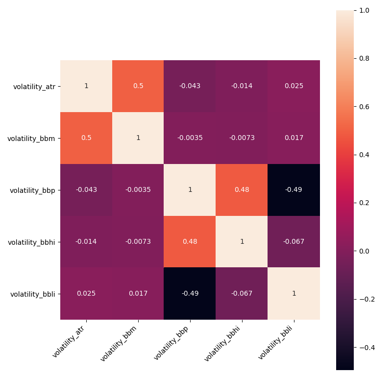
Before calculating the volatility heatmap, there were five indicators. As a result, we see the exact count of indicators. These are excellent results, which means that all our indicators are calculated using different techniques that give us such uncorrelated features. This means that none of all volatility indicators were correlating.

Volume indicators

The third batch is well-known volume indicators. The volume shows us the number of shares security has been traded in a given period. Volume indicators are simple mathematical formulas that are visually represented in most commonly used trading platforms. Same way as before, I created a function that we will use to get a Heatmap of the volume indicators:

def get_volume_indicators(df, threshold=0.5, plot=False):
    df_volume = df.copy()
    
    # add custom volume indicators
    # ...

    df_volume = add_volume_ta(df_volume, high="High", low="Low", close="Close", volume="Volume")

    return DropCorrelatedFeatures(df_volume, threshold, plot)

We run this above function in the following way:

df = pd.read_csv('./BTCUSD_1h.csv')
df = df.sort_values('Date')
get_volume_indicators(df, threshold=0.5, plot=True)

Matplotlib should give us the following results:

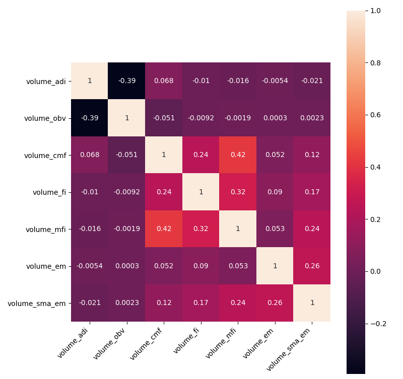
Before calculating the heatmap, there were nine indicators. After dropping correlated ones, there left 7 of them. This means that only 22% of all volume indicators were correlating. That's an impressive result, even now, we can see that we could decrease the threshold, but the count of indicators will stay the same because they are highly uncorrelated.

Momentum indicators

Momentum indicators show the movement of the price over time and how strong those movements were, are or will be, regardless of the direction the price is moving. It is said that momentum indicators are also helpful because they help traders and analysts recognize points where the market might reverse. We add these indicators with the following function:

def get_momentum_indicators(df, threshold=0.5, plot=False):
    df_momentum = df.copy()
    
    # add custom momentum indicators
    # ...

    df_momentum = add_momentum_ta(df_momentum, high="High", low="Low", close="Close", volume="Volume")

    return DropCorrelatedFeatures(df_momentum, threshold, plot)

We run this above function in the following way:

df = pd.read_csv('./BTCUSD_1h.csv')
df = df.sort_values('Date')
get_momentum_indicators(df, threshold=0.5, plot=True)

Matplotlib should give us the following results:

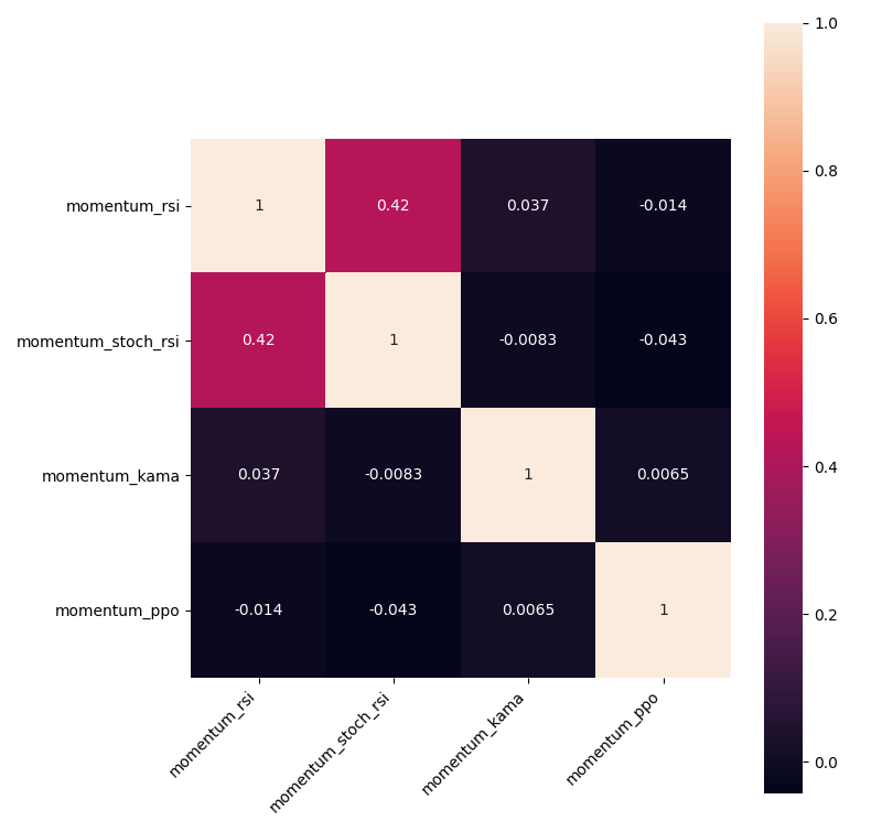
Before calculating the heatmap, there were 11 indicators; after dropping correlated ones, there left only 4 of them. This means that 64% of all momentum indicators were correlating. This implies that momentum indicators are the most correlated.

Other indicators

The last batch of indicators is Daily Return (DR), Daily Log Return (DLR), Cumulative Return (CR). I am not sure what they are about, but anyway, I don't see a reason why we shouldn't add them to our model with the following function:

def get_others_indicators(df, threshold=0.5, plot=False):
    df_others = df.copy()
    
    # add custom indicators
    # ...

    df_others = add_others_ta(df_others, close="Close")

    return DropCorrelatedFeatures(df_others, threshold, plot)

We run this above function in the following way:

df = pd.read_csv('./BTCUSD_1h.csv')
df = df.sort_values('Date')
get_others_indicators(df, threshold=0.5, plot=True)

Matplotlib should give us the following results:

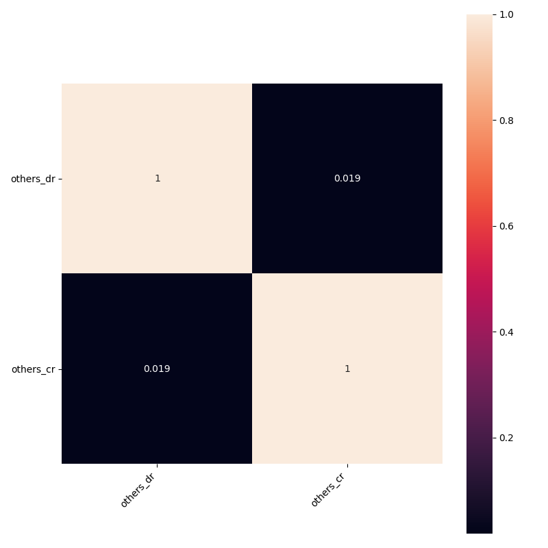
There is nothing much to say about this because there were only three indicators, and one of them was highly correlated. In case you want to calculate the correlation between all indicators without separating them into different groups, you may run the following function:

def get_all_indicators(df, threshold=0.5, plot=False):
    df_all = df.copy()
    
    # add custom indicators
    # ...

    df_all = add_all_ta_features(df_all, open="Open", high="High", low="Low", close="Close", volume="Volume")

    return DropCorrelatedFeatures(df_all, threshold, plot)

Everything is quite the same as before.

So, now, when we have all the functions needed to calculate and drop correlation from each indicator group, we need to run the following function:

def indicators_dataframe(df, threshold=0.5, plot=False):
    trend       = get_trend_indicators(df, threshold=threshold, plot=plot)
    volatility  = get_volatility_indicators(df, threshold=threshold, plot=plot)
    volume      = get_volume_indicators(df, threshold=threshold, plot=plot)
    momentum    = get_momentum_indicators(df, threshold=threshold, plot=plot)
    others      = get_others_indicators(df, threshold=threshold, plot=plot)
    #all_ind = get_all_indicators(df, threshold=threshold)

    final_df = [df, trend, volatility, volume, momentum, others]
    result = pd.concat(final_df, axis=1)

    return result

The above function will merge all our indicators into one beautiful panda's data frame, which we'll use further for our RL Bitcoin trading bot model.

Before moving ahead, I would like to come back to normalization. As I mentioned initially, I offered another normalization method that we will use to normalize indicators. But here comes another problem: our indicators might have negative values, and when we try to apply the logarithm to these negative values, we get a NaN result. So I decided not to use logarithm if the resulting values are negative with the following function:

def Normalizing(df_original):
    df = df_original.copy()
    column_names = df.columns.tolist()
    for column in column_names[1:]:
        # Logging and Differencing
        test = np.log(df[column]) - np.log(df[column].shift(1))
        if test[1:].isnull().any():
            df[column] = df[column] - df[column].shift(1)
        else:
            df[column] = np.log(df[column]) - np.log(df[column].shift(1))
        # Min Max Scaler implemented
        Min = df[column].min()
        Max = df[column].max()
        df[column] = (df[column] - Min) / (Max - Min)

    return df

Training and testing

Because I changed how we insert indicators into our dataset and how we normalize our dataset, there were a lot of places where I made small code changes. I decided not to mention these changes in this tutorial because this tutorial would be only about changes. But I will introduce the most extensive changes.

When we were starting to train our model in all previous tutorial series parts, all parameters were written into a parameters.txt file. I decided instead of writing simply into txt, do it in JSON structure:

def start_training_log(self, initial_balance, normalize_value, train_episodes):      
    # save training parameters to Parameters.json file for future
    current_date = datetime.now().strftime('%Y-%m-%d %H:%M')
    params = {
        "training start": current_date,
        "initial balance": initial_balance,
        "training episodes": train_episodes,
        "lookback window size": self.lookback_window_size,
        "depth": self.depth,
        "lr": self.lr,
        "epochs": self.epochs,
        "batch size": self.batch_size,
        "normalize value": normalize_value,
        "model": self.model,
        "comment": self.comment,
        "saving time": "",
        "Actor name": "",
        "Critic name": "",
    }
    with open(self.log_name+"/Parameters.json", "w") as write_file:
        json.dump(params, write_file, indent=4)

While using JSON structure, it's much easier for us to load our training setting when we want to test a particular model that we trained in the past. So, this JSON improvement led me to change test_agent and test_multiprocessing functions. Now we'll need only to call them with fewer parameters.

I received many comments in my previous tutorials that I am not considering order fees while making trades. I decided that it's an excellent place to add this finally. So I made small changes in my step function:

def step(self, action):
    ...
    if action == 0: # Hold
        pass

    elif action == 1 and self.balance > self.initial_balance*0.05:
        # Buy with 100% of current balance
        self.crypto_bought = self.balance / current_price
        self.crypto_bought *= (1-self.fees) # substract fees
        self.balance -= self.crypto_bought * current_price
        self.crypto_held += self.crypto_bought
        self.trades.append({'Date' : Date, 'High' : High, 'Low' : Low, 'total': self.crypto_bought, 'type': "buy", 'current_price': current_price})
        self.episode_orders += 1

    elif action == 2 and self.crypto_held*current_price> self.initial_balance*0.05:
        # Sell 100% of current crypto held
        self.crypto_sold = self.crypto_held
        self.crypto_sold *= (1-self.fees) # substract fees
        self.balance += self.crypto_sold * current_price
        self.crypto_held -= self.crypto_sold
        self.trades.append({'Date' : Date, 'High' : High, 'Low' : Low, 'total': self.crypto_sold, 'type': "sell", 'current_price': current_price})
        self.episode_orders += 1

You might see that there are two new lines:

• self.crypto_bought *= (1-self.fees) when we do buy action;
• self.crypto_sold *= (1-self.fees) when we do sell action.

In both actions, we subtract fees from our balance, whether held in crypto or cash. In most exchanges, this fee is around 0.1%, but if you need it, you can search for the self.fees line in code and change to whatever you want.

Also, you may notice that I removed all the stuff related to punish_value, which was used to motivate our bot to make trades instead of holding bitcoin until the end.

Now, because I use a lot of indicators, data preparation is much more complex, the example you can see below:

if __name__ == "__main__":            
    df = pd.read_csv('./BTCUSD_1h.csv')
    df = df.dropna()
    df = df.sort_values('Date')

    #df = AddIndicators(df) # insert indicators to df
    df = indicators_dataframe(df, threshold=0.5, plot=False) # insert indicators to df
    depth = len(list(df.columns[1:])) # OHCL + indicators without Date

    df_nomalized = Normalizing(df[99:])[1:].dropna() # we cut first 100 bars to have properly calculated indicators
    df = df[100:].dropna() # we cut first 100 bars to have properly calculated indicators

    lookback_window_size = 100
    test_window = 720*3 # 3 months
    
    # split training and testing datasets
    train_df = df[:-test_window-lookback_window_size]
    test_df = df[-test_window-lookback_window_size:]
    
    # split training and testing normalized datasets
    train_df_nomalized = df_nomalized[:-test_window-lookback_window_size]
    test_df_nomalized = df_nomalized[-test_window-lookback_window_size:]

    # multiprocessing training/testing. Note - run from cmd or terminal
    agent = CustomAgent(lookback_window_size=lookback_window_size, lr=0.00001, epochs=5, optimizer=Adam, batch_size=32, model="CNN", depth=depth, comment="Normalized")
    train_multiprocessing(CustomEnv, agent, train_df, train_df_nomalized, num_worker = 32, training_batch_size=500, visualize=False, EPISODES=400000)
    
    test_multiprocessing(CustomEnv, CustomAgent, test_df, test_df_nomalized, num_worker = 16, visualize=False, test_episodes=1000, folder="2021_02_11_15_40_Crypto_trader", name="", comment="")

Instead of calling the AddIndicators function, now I run the indicators_dataframe function, which in the current example adds 30 different indicators. I call this indicators_count - depth that we use to construct the right state_size of our model.

You might see that now we have train_df and train_df_normalized data frames. Train_df is without normalization — mainly is used only while rendering beautiful visualization and calculating rewards while our model is training. Train_df_normalized is normalized data that we use only for training.

We need to create an agent with CustomAgent class with our parameters and feed everything to train_multiprocessing functions to start the training process.

I trained an agent with the same parameters that I used in my previous tutorial to compare any performance improvement coming from more indicators and a new normalization technique. Here is my Parameters.json file with all our indicators of the 2021_02_18_21_48_Crypto_trader model:

{
 “training start”: “2021–02–18 21:48”,
 “initial balance”: 1000,
 “training episodes”: 400000,
 “lookback window size”: 100,
 “depth”: 30,
 “lr”: 1e-05,
 “epochs”: 5,
 “batch size”: 32,
 “normalize value”: 40000,
 “model”: “CNN”,
 “comment”: “Normalized, no punish value”,
 “saving time”: “2021–02–21 05:09”,
 “Actor name”: “3906.52_Crypto_trader_Actor.h5”,
 “Critic name”: “3906.52_Crypto_trader_Critic.h5”
}

That's right; I trained the model for 400k training steps, which took around 55 hours. The best model was named 3906.52_Crypto_trader and testing results for three months were: 1162.08$ at the end, that's not that nice as I expected. I made a chart where I show rewards, episode orders, and no profit episodes for each month:

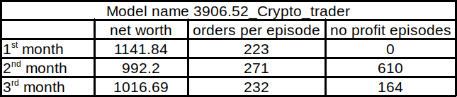
As we can see, we made a profit in the first month, but another two months were not that great. Even if there was a downtrend, we want that our bot could deal with it.

Then I decided to train another model by using AddIndicators instead of the indicators_dataframe function as in the previous tutorial. The only difference from the previous tutorial will be that now we'll use a new normalization technique. Here is my Parameters.json file with all our indicators of the 2021_02_21_17_54_Crypto_trader model:

{
 “training start”: “2021–02–21 17:54”,
 “initial balance”: 1000,
 “training episodes”: 400000,
 “lookback window size”: 100,
 “depth”: 13,
 “lr”: 1e-05,
 “epochs”: 5,
 “batch size”: 32,
 “normalize value”: 40000,
 “model”: “CNN”,
 “comment”: “Normalized, no punish value”,
 “saving time”: “2021–02–23 11:44”,
 “Actor name”: “3263.63_Crypto_trader_Actor.h5”,
 “Critic name”: “3263.63_Crypto_trader_Critic.h5”
}

As you can see, now depth is 13, not 30, and training took less time (42 hours). Within the same testing dataset of 3 months, we had 1478.50$ net worth in balance at the end of testing results. This is quite similar to the previous tutorial. Here is a similar chart of 3 months as before:

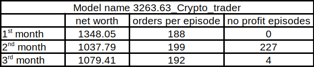
I assume that too many indicators added to our model create noise to our training data so that our model can't learn market price action. This is why our bot performs better with fewer indicators than more. Here is a similar comparison of our previous tutorial model with the same training and testing dataset:

As we can see, our previous model performed a little better because it had fewer profit episodes during the testing timeframe and the total net worth was also a little better.

Anyway, I think that the current model with fewer indicators performs better. Because we used a new normalization technique to remove trends from our data, our model doesn't learn to trade only Bitcoin. Our model could probably even trade profitably another market pair, which we need to test, but this is not the subject of this tutorial.

This is how our 2021_02_21_17_54_Crypto_trader bot looks while trading on unseen data:

It's pretty impressive how it performs while there is an uptrend or when the market goes sideways. I am happy that it even learned to avoid dips. But it's not that good when the short-term trend is going down, but the reason might be because Bitcoin, looking at the long term, mostly goes only to up direction.

Conclusion:

We learned from this tutorial that more technical indicators don't mean that they always will give us a better performance of our RL Bitcoin trading bot. This is because most of the indicators are lagging, adding too much noise to our training dataset.

The bigger picture of what we achieved from developing random trading agents in my first tutorial and seeing it now has impressive results. Speaking openly, while doing this tutorial, I didn't even expect that it's possible to beat the market and make this kind of automation bot do trades profitably.

Of course, this bot is not perfect. Experienced automated bot coders might give me a lot of advice on where and how to improve it. Still, results exceeded my expectations because I developed and researched this by myself in my spare time!

This tutorial code can be copied and used wherever you want, but I do not recommend using it for actual trading because you might lose all your money, don't blame me for that if you do so! Anyway, this whole stuff with reinforcement learning required too much effort, time, and knowledge. This means that this is my last Bitcoin trading tutorial part, and I might not come back to it quite soon. I never say never, but I still need more Reinforcement Learning and more profound Machine Learning knowledge to achieve better results!

For now, I'll continue researching other Python and Machine learning spheres; if you are interested, you can follow me.

Thanks for reading! As always, all the code given in this tutorial can be found on my GitHub page and is free to use!

All of these tutorials are for educational purposes and should not be taken as trading advice. It would be best to not trade based on any algorithms or strategies defined in this, previous, or future tutorials, as you are likely to lose your investment.