In this tutorial, we will continue developing a Bitcoin trading bot, but this time instead of making trades randomly, we'll use the power of reinforcement learning.
The purpose of the previous and this tutorial is to experiment with state-of-the-art deep reinforcement learning technologies to see if we can create a profitable Bitcoin trading bot. Many articles on the internet state that Neural Networks can't beat the market. However, recent advances in the field have shown that RL agents are often capable of learning much more than supervised learning agents within the same problem domain. For this reason, I am writing these tutorials to experiment, if possible, and if it is, how profitable we can make these trading bots.
While I won't be creating anything quite as impressive as OpenAI engineers did, it is still not an easy task to trade Bitcoin profitably on a day-to-day basis and do it at a profit!
Plan up to this point

Before moving forward, we'll cover what we must do to achieve our goal:
- Create a custom trading environment for our Agent to learn from;
- Render a simple and elegant visualization of that environment;
- Train our Reinforcement Learning agent to learn a profitable trading strategy (Current);
If you are not already familiar with my previous tutorials, create a custom crypto trading environment from scratch — Bitcoin trading bot example and Visualize an elegant Bitcoin RL trading agent chart using Matplotlib. Not so long ago, I wrote tutorials on both of those topics. Feel free to pause here and read either of those before continuing with this (third) tutorial.
Implementation
I will use the same market history data that I used in my previous tutorial for this tutorial. If you missed where I got it, here is the link https://bitcoincharts.com/. The .csv file will also be available on my GitHub repository along with this complete tutorial code. If you want to test it out before testing, I recommend reading this tutorial. Okay, let's get started.
While writing code in this tutorial, I thought that for people who are beginners in Python might be complicated with required libraries, so I decided to add a requirements.txt file to my GitHub repository, so people would know what packages they need to install. So, if you clone my code, before testing it, make sure to run pip install -r ./requirements.txt command, that will install all required packages for this tutorial:
numpy
tensorflow==2.3.1
tensorflow-gpu==2.3.1
opencv-python
matplotlib
tensorboardx
pandas
mplfinance
I want to say that this (Third) tutorial part will require little custom programming creativity. I already have programmed everything we need in the past. I need to merge two different codes with slight modifications. If you were following me, I already wrote and tested Proximal Policy Optimization (PPO) reinforcement learning agent for the Gym LunarLander-v2 environment. So, I will need to pick that code and merge it with my previous tutorial code.
If you are not familiar with PPO, I recommend reading my previous LunarLander-v2 tutorial. This will help you to form an idea of what we are doing here. Different from my previous tutorial, I'll define my model architecture in another file called model.py. So I copy Actor_Model and Critic_Model classes to the following file, and at the beginning of the file, I add all necessary imports to build our code:
import numpy as np
import tensorflow as tf
from tensorflow.keras.models import Model
from tensorflow.keras.layers import Input, Dense, Flatten
from tensorflow.keras import backend as K
#tf.config.experimental_run_functions_eagerly(True) # used for debuging and development
tf.compat.v1.disable_eager_execution() # usually using this for fastest performance

gpus = tf.config.experimental.list_physical_devices('GPU')
if len(gpus) > 0:
    print(f'GPUs {gpus}')
    try: tf.config.experimental.set_memory_growth(gpus[0], True)
    except RuntimeError: pass

class Actor_Model:
    def __init__(self, input_shape, action_space, lr, optimizer):
        X_input = Input(input_shape)
        self.action_space = action_space

        X = Flatten(input_shape=input_shape)(X_input)
        X = Dense(512, activation="relu")(X)
        X = Dense(256, activation="relu")(X)
        X = Dense(64, activation="relu")(X)
        output = Dense(self.action_space, activation="softmax")(X)

        self.Actor = Model(inputs = X_input, outputs = output)
        self.Actor.compile(loss=self.ppo_loss, optimizer=optimizer(lr=lr))

    def ppo_loss(self, y_true, y_pred):
        # Defined in https://arxiv.org/abs/1707.06347
        advantages, prediction_picks, actions = y_true[:, :1], y_true[:, 1:1+self.action_space], y_true[:, 1+self.action_space:]
        LOSS_CLIPPING = 0.2
        ENTROPY_LOSS = 0.001

        prob = actions * y_pred
        old_prob = actions * prediction_picks

        prob = K.clip(prob, 1e-10, 1.0)
        old_prob = K.clip(old_prob, 1e-10, 1.0)

        ratio = K.exp(K.log(prob) - K.log(old_prob))

        p1 = ratio * advantages
        p2 = K.clip(ratio, min_value=1 - LOSS_CLIPPING, max_value=1 + LOSS_CLIPPING) * advantages

        actor_loss = -K.mean(K.minimum(p1, p2))

        entropy = -(y_pred * K.log(y_pred + 1e-10))
        entropy = ENTROPY_LOSS * K.mean(entropy)

        total_loss = actor_loss - entropy

        return total_loss

    def predict(self, state):
        return self.Actor.predict(state)

class Critic_Model:
    def __init__(self, input_shape, action_space, lr, optimizer):
        X_input = Input(input_shape)

        V = Flatten(input_shape=input_shape)(X_input)
        V = Dense(512, activation="relu")(V)
        V = Dense(256, activation="relu")(V)
        V = Dense(64, activation="relu")(V)
        value = Dense(1, activation=None)(V)

        self.Critic = Model(inputs=X_input, outputs = value)
        self.Critic.compile(loss=self.critic_PPO2_loss, optimizer=optimizer(lr=lr))

    def critic_PPO2_loss(self, y_true, y_pred):
        value_loss = K.mean((y_true - y_pred) ** 2) # standard PPO loss
        return value_loss

    def predict(self, state):
        return self.Critic.predict([state, np.zeros((state.shape[0], 1))])
As I said, I will not explain how the PPO model works because that's already covered. But you might notice one difference in code, instead of using X = Dense(512, activation=”relu”)(X_input) as input, I use X = Flatten(input_shape=input_shape)(X_input). I do so because our model input shape is 3D of shape (1, 50, 10), and our first Dense layer doesn't understand this, so I use the Flatten layer, which gives me a concatenated array of shape (1, 500) — this is the value our model will try to learn from.
Ok, coming back to my main script, there are also many upgrades. First of all to existing imports I add three more:
from tensorboardX import SummaryWriter
from tensorflow.keras.optimizers import Adam, RMSprop
from model import Actor_Model, Critic_Model
TensorboardX will be used for our Tensorboard logs, you may use it or not, it's up to you, but sometimes it's useful. Next, I import Adam and RMSprop optimizers for our experimentations to change and experiment with different optimizers from the main script. And lastly, I'll import our newly created Actor and Critic classes.
In the main script, to our CustomEnv class init part, I add the following code:
def __init__(self, df, initial_balance=1000, lookback_window_size=50, Render_range = 100):
    ...

    # Neural Networks part bellow
    self.lr = 0.0001
    self.epochs = 1
    self.normalize_value = 100000
    self.optimizer = Adam

    # Create Actor-Critic network model
    self.Actor = Actor_Model(input_shape=self.state_size, action_space = self.action_space.shape[0], lr=self.lr, optimizer = self.optimizer)
    self.Critic = Critic_Model(input_shape=self.state_size, action_space = self.action_space.shape[0], lr=self.lr, optimizer = self.optimizer)

    # create tensorboard writer
    def create_writer(self):
        self.replay_count = 0
        self.writer = SummaryWriter(comment="Crypto_trader")
Here I define learning rate, training epochs, and chosen Optimizer for our neural network. Also, here I define normalization/scaling value that is typically recommended and sometimes very important. Especially for neural networks, normalization can be very crucial because when we input unnormalized inputs to activation functions, we can get stuck in a very flat region in the domain and may not learn at all. Or worse, we end up with numerical issues. I would need to get deeper into this normalization stuff later, but now I will use the value of 100000 because I know there is no bigger number in my dataset. In the best case, we should use normalization values between min and max, but what's if our future market highs get bigger than we had in our history? Actually, with normalization, I have more questions than answers that I will need to answer in the future. Now I'll use this hardcoded normalization.
Although we create our Actor and Critic classes in this place, that will do all the complex works for us! The replay counter and writer are used for our Tensorboard logging stuff; nothing so important.
Next, I copied replay, act, save and load functions. All of them didn't change. Except for replay, I added three lines used for my Tensorboard writer to log our actor and critic losses at the end of it. Also, I forgot to mention that in the reset function, I added a self.episode_orders parameter, which I use in the step function. Every time our Agent does sell or buy orders, I increment self.episode_orders by one; I use this parameter to track how many orders the Agent does through one episode.
Training the Agent
How do we train this Agent to make profitable trades in the market? I think this part is one of the most waited. Usually, every newcomer to reinforcement learning doesn't know how to prepare their Agent to solve their problem in a concrete environment, so I recommend starting from simple problems and doing small steps while trying more difficult environments by getting better scores. So this is the reason why I implemented random trading in my first tutorial. Now we can use it to build on top of it, to give our Agent some reasonable actions. So here is our code to train the Agent:
def train_agent(env, visualize=False, train_episodes = 50, training_batch_size=500):
    env.create_writer() # create TensorBoard writer
    total_average = deque(maxlen=100) # save recent 100 episodes net worth
    best_average = 0 # used to track best average net worth
    for episode in range(train_episodes):
        state = env.reset(env_steps_size = training_batch_size)

        states, actions, rewards, predictions, dones, next_states = [], [], [], [], [], []
        for t in range(training_batch_size):
            env.render(visualize)
            action, prediction = env.act(state)
            next_state, reward, done = env.step(action)
            states.append(np.expand_dims(state, axis=0))
            next_states.append(np.expand_dims(next_state, axis=0))
            action_onehot = np.zeros(3)
            action_onehot[action] = 1
            actions.append(action_onehot)
            rewards.append(reward)
            dones.append(done)
            predictions.append(prediction)
            state = next_state

        env.replay(states, actions, rewards, predictions, dones, next_states)
        total_average.append(env.net_worth)
        average = np.average(total_average)

        env.writer.add_scalar('Data/average net_worth', average, episode)
        env.writer.add_scalar('Data/episode_orders', env.episode_orders, episode)

        print("net worth {} {:.2f} {:.2f} {}".format(episode, env.net_worth, average, env.episode_orders))
        if episode > len(total_average):
            if best_average < average:
                best_average = average
                print("Saving model")
                env.save()
Also, I am not going to explain the training part step by step. If you want to understand all steps here, check my reinforcement learning tutorials. But I will give short notices. I use the following lines to plot our net worth average and how many orders our Agent does through the episode:
env.writer.add_scalar('Data/average net_worth', average, episode)
env.writer.add_scalar('Data/episode_orders', env.episode_orders, episode)
The above lines will help us to see how our Agent is learning stuff. Also, instead of saving our model every step, I track the best average score our model could achieve through 100 episodes and keep only the best one. Also, I am not sure if this is a suitable evaluation method, but we'll see.
Testing the Agent
Testing the Agent is just as important as training, or even more relevant, so we need to know how to test our Agent. Test agent function is very similar to our random games agent:
def test_agent(env, visualize=True, test_episodes=10):
    env.load() # load the model
    average_net_worth = 0
    for episode in range(test_episodes):
        state = env.reset()
        while True:
            env.render(visualize)
            action, prediction = env.act(state)
            state, reward, done = env.step(action)
            if env.current_step == env.end_step:
                average_net_worth += env.net_worth
                print("net_worth:", episode, env.net_worth, env.episode_orders)
                break

    print("average {} episodes agent net_worth: {}".format(test_episodes, average_net_worth/test_episodes))
There are only two differences:
- At the beginning of the function, we load our trained model weights;
- Second, instead of making random actions
(action = np.random.randint(3, size=1)[0])we use a trained model to predict the action(action, prediction = env.act(state));
The fun begins - the training part:
One of the biggest mistakes others make while writing market prediction scripts is that they do not split the data into a training and test set. I think that it's evident that the model will perform nicely on seen data. The purpose of separating the dataset into training and testing is to test the accuracy of our final model on new data it has never seen before. Since we are using time series data, we don't have many options for cross-validation.
For example, one common form of cross-validation is called k-fold validation. Data is split into k equal groups and one by one single out a group as the test group, and the rest of the information is used as the training group. However, time-series data is highly time-dependent, meaning later data is highly dependent on previous data. So k-fold won't work because our Agent will learn from future data before trading it; that's an unfair advantage.
So, we are left with taking a slice of the entire data frame to use as the training set from the beginning of the frame up to some arbitrary index and using the rest of the data as the test set:
df = pd.read_csv(‘./pricedata.csv’)
df = df.sort_values(‘Date’)
lookback_window_size = 50
train_df = df[:-720-lookback_window_size]
test_df = df[-720-lookback_window_size:] # 30 days
Since our environment is only set up to handle a single data frame, we are creating two environments, one for the training data and one for the test data:
train_env = CustomEnv(train_df,lookback_window_size=lookback_window_size)
test_env = CustomEnv(test_df,lookback_window_size=lookback_window_size)
Now, training our model is as simple as creating an agent with our environment and calling the above-created training function:
train_agent(train_env, visualize=False, train_episodes=20000, training_batch_size=500)I am not sure how long I should train it, but I chose to train for 20k steps. Let's see how our training process looks in Tensorboard by writing the following command in the terminal: tensorboard --logdir runs and opening http://localhost:6006/ in our browser.
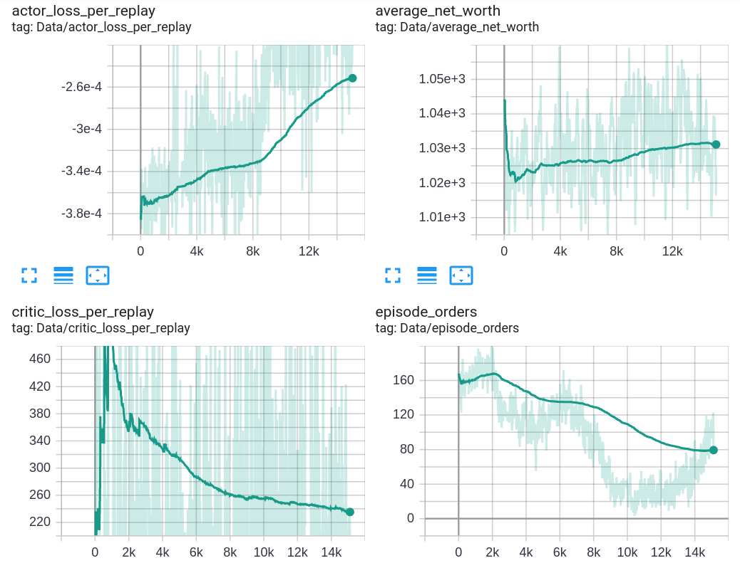
The above image shows my Tensorboard results while I was training our Agent for 20k training episodes. As you can see, it's okay that actor loss goes up and critic loss goes down and stabilizes through time. But one of the most exciting charts for me is episode orders and average net worth. Yes, we can see that our average net worth goes up, but only by a few percent from the initial balance - but still, that's a profit! The above graphs tell us that our Agent is learning, and as you can see, Agent thought that it's better to do fewer orders than more. At one training moment, the agent event brought that the best trading strategy is holding, but we don't want to do that. What I tried to answer from the above chart is, can our Agent learn something? The answer was — YES! I am 100% sure we can say YES; our Agent is learning something, but it's pretty hard to tell what.
Test with unseen data
At first, let's see how the agent performs on data, which it never seen before:
This is only a short GIF, but if you want to see more, the best is to watch my YouTube video, where I show and explain everything, or you can clone my GitHub repository and test this Agent by yourself.
Ok, let’s evaluate our agent, and let's check if we can beat a random agent for 1000 episode steps with the following two commands:
test_agent(test_env, visualize=False, test_episodes=1000)
Random_games(test_env, visualize=False, train_episodes = 1000)
And here are the results of our trained Agent:
average 1000 episodes agent net_worth: 1043.4012850463675
And here are our random agent results:
average 1000 episodes random net_worth: 1024.3194149765457
The only reason why our random Agent also got a nice profit is that our market trend was up. Considering that this average profit of our Agent was made in one month, 4% sounds like a pretty nice result. But also, seeing my trading agent gif above, its behavior is quite strange; an agent doesn't like holding zero-orders. However, I noticed that Agent, just after selling all open positions, quickly opens another buy. This would never lead us to good profits, so we'll need to analyze and solve this problem.
Conclusion:
This was quite a long tutorial, and we'll stop here. We achieved our goal to create a profitable Bitcoin trading agent from scratch, using deep reinforcement learning, to beat the market! We have already accomplished the following:
- Made a Bitcoin trading environment from scratch;
- Built a rendered visualization of that environment;
- Trained and tested our Agent with unseen data;
- Our Agent performed a little better than the random Agent and made some profit!
While our trading agent isn't quite as profitable as we'd hoped, it is getting somewhere. I am not sure what I'll try to do in the next tutorial, but I am sure that I'll test some different reward strategies, maybe will do some model optimizations. But we all know that we must get better profits on unseen data, so I'll work on it!
Thanks for reading! See you in the next part, where we'll try to use more techniques to improve our Agent! As always, all the code given in this tutorial can be found on my GitHub page and is free to use!
All of these tutorials are for educational purposes and should not be taken as trading advice. It would be best to not trade based on any algorithms or strategies defined in this, previous, or future tutorials, as you are likely to lose your investment.