Let's improve our deep RL Bitcoin trading agent code to make even more money with a better reward strategy and test different model structures.

In the previous tutorial, we used deep reinforcement learning to create a Bitcoin trading agent that could beat the market. Although our agent was profitable compared to random actions, the results weren't all that impressive, so this time, we're going to step it up, and we'll try to implement a few more improvements with the reward system. We'll test how our profitability depends on the Neural Network model structure. Although, we'll test everything with our code, and of course, you'll be able to download everything from my GitHub repository.

Reward Optimization

While writing my reward strategy, I would like to mention that it was pretty hard to find what reward strategies others use in reinforcement learning while implementing automated trading strategies. It's pretty hard to see what others do, and if I could find it, these strategies were poorly documented and quite complicated to understand. I believe that there are a lot of exciting and successful strategy solutions, but for this tutorial, I decided to rely on my intuition and try my strategy.

Someone might think that our reward function from the previous tutorial (i.e., calculating the change in net worth at each step) is the best we can do. But that is far from the truth. While our simple reward feature may have made a small profit last time, it will often lead us to losses in the capital. To improve this, in addition to simply unrealized gains, we will have to consider other reward metrics.

The main improvement that comes to my head is that we must reward profits from holding BTC while increasing in price and reward profits from not holding BTC while the price is decreasing. One of the ideas is that we can reward our agent for any gradual increase in net-worth while holding a BTC/USD position and again reward it for the cumulative decrease in value of BTC/USD while not having any open positions.

Although, we'll implement this by calculating our reward when we sell our held Bitcoins or buy Bitcoin after our price drops. Between orders, while our agent does nothing, we won't use any rewards because these rewards are calculated with a discount function. So, when I used this reward strategy, I noticed that my agent usually learns to hold instead of learning to do profitable orders, so I decided to punish it for doing nothing. I subtract 0.01% of net worth every step. This way, our agent learned that it's not the best idea to keep holding Bitcoin or open positions forever. Also, the agent understood that sometimes it's better to cut the loss and wait for another opportunity to make an order.

So here is my code of the custom reward function:

# Calculate reward
def get_reward(self):
    self.punish_value += self.net_worth * 0.00001
    if self.episode_orders > 1 and self.episode_orders > self.prev_episode_orders:
        self.prev_episode_orders = self.episode_orders
        if self.trades[-1]['type'] == "buy" and self.trades[-2]['type'] == "sell":
            reward = self.trades[-2]['total']*self.trades[-2]['current_price'] - self.trades[-2]['total']*self.trades[-1]['current_price']
            reward -= self.punish_value
            self.punish_value = 0
            self.trades[-1]["Reward"] = reward
            return reward
        elif self.trades[-1]['type'] == "sell" and self.trades[-2]['type'] == "buy":
            reward = self.trades[-1]['total']*self.trades[-1]['current_price'] - self.trades[-2]['total']*self.trades[-2]['current_price']
            reward -= self.punish_value
            self.trades[-1]["Reward"] = reward
            self.punish_value = 0
            return reward
    else:
        return 0 - self.punish_value

Suppose you are reading this tutorial without getting familiar with my previous tutorial or complete code. In that case, you probably can't understand this code, so check my code on GitHub or previous tutorials to get familiar with it.

As you can see from the above code, the first thing we do, we calculate the punishing value that is cumulative every step. If orders are made, we set it to zero. If we looked at the if statements, we would see two of them: buying just after sell, and wise versa. You may ask, why sometimes I use self.trades[-2] and sometimes self.trades[-1]. This is done because we want to calculate the reward of orders that are not open. Because we can't make an actual profit when we sell our Bitcoin and buy later (except margin trading), but in the above way, we can calculate what we didn't lose while selling high and buying low.

While I was developing this strategy, it was pretty tricky to understand if I implemented it correctly, so I decided to improve our render function in utils.py with the following code:

# sort sell and buy orders, put arrows in appropiate order positions
for trade in trades:
    trade_date = mpl_dates.date2num([pd.to_datetime(trade['Date'])])[0]
    if trade_date in Date_Render_range:
        if trade['type'] == 'buy':
            high_low = trade['Low']-10
            self.ax1.scatter(trade_date, high_low, c='green', label='green', s = 120, edgecolors='none', marker="^")
        else:
            high_low = trade['High']+10
            self.ax1.scatter(trade_date, high_low, c='red', label='red', s = 120, edgecolors='none', marker="v")

To more dynamic code:

minimum = np.min(np.array(self.render_data)[:,1:])
maximum = np.max(np.array(self.render_data)[:,1:])
RANGE = maximum - minimum

# sort sell and buy orders, put arrows in appropiate order positions
for trade in trades:
    trade_date = mpl_dates.date2num([pd.to_datetime(trade['Date'])])[0]
    if trade_date in Date_Render_range:
        if trade['type'] == 'buy':
            high_low = trade['Low'] - RANGE*0.02
            ycoords = trade['Low'] - RANGE*0.08
            self.ax1.scatter(trade_date, high_low, c='green', label='green', s = 120, edgecolors='none', marker="^")
        else:
            high_low = trade['High'] + RANGE*0.02
            ycoords = trade['High'] + RANGE*0.06
            self.ax1.scatter(trade_date, high_low, c='red', label='red', s = 120, edgecolors='none', marker="v")

        if self.Show_reward:
            try:
                self.ax1.annotate('{0:.2f}'.format(trade['Reward']), (trade_date-0.02, high_low), xytext=(trade_date-0.02, ycoords),
                                           bbox=dict(boxstyle='round', fc='w', ec='k', lw=1), fontsize="small")
            except:
                pass

As you can see, now, instead of using hardcoded offset withing high_low, I calculate that range - this way, we could use the same rendering graph for different trading pairs (not tested yet) without modifying our offset. But most importantly, I am adding the reward number below the buy order arrow and above the sell order arrow - this helped me to understand if I implemented my reward function correctly, take a look at it:

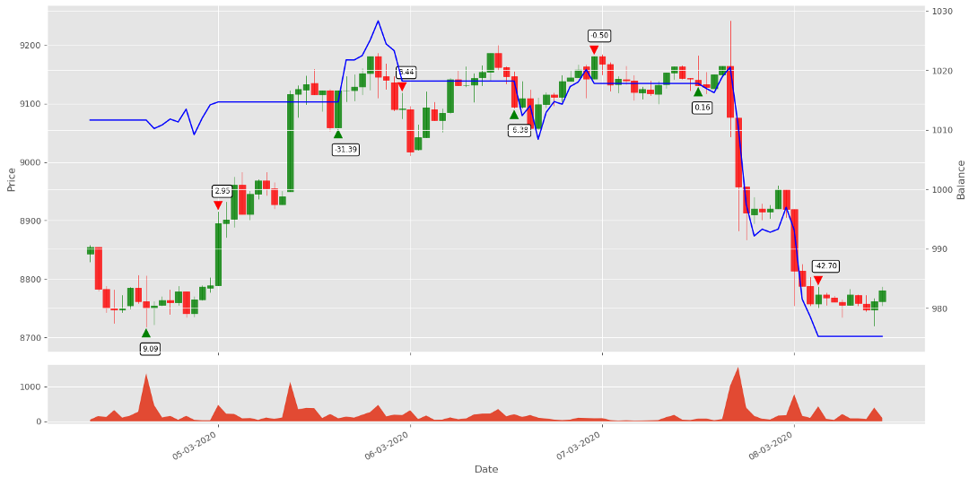Looking at this chart, it's pretty obvious where our agent did good orders and where they are terrible. This is the information we'll use to train our agent.

Model modifications

We probably know that our decisions mainly depend on our knowledge of what good or bad decisions we make in our lives, how fast we are learning new stuff, and the list can continue. All of this depends on our brain functionality. The same is with the model; everything depends on our brains and how well it is trained. The biggest problem is that we don't know what architecture we should use for our model to beat the market. The only way left is to try different architectures.

We already use a Dense basic layer for our Actor and Critic neural networks:

# Critic model
X = Flatten()(X_input)
V = Dense(512, activation="relu")(X)
V = Dense(256, activation="relu")(V)
V = Dense(64, activation="relu")(V)
value = Dense(1, activation=None)(V)

# Actor model
X = Flatten()(X_input)
A = Dense(512, activation="relu")(X)
A = Dense(256, activation="relu")(A)
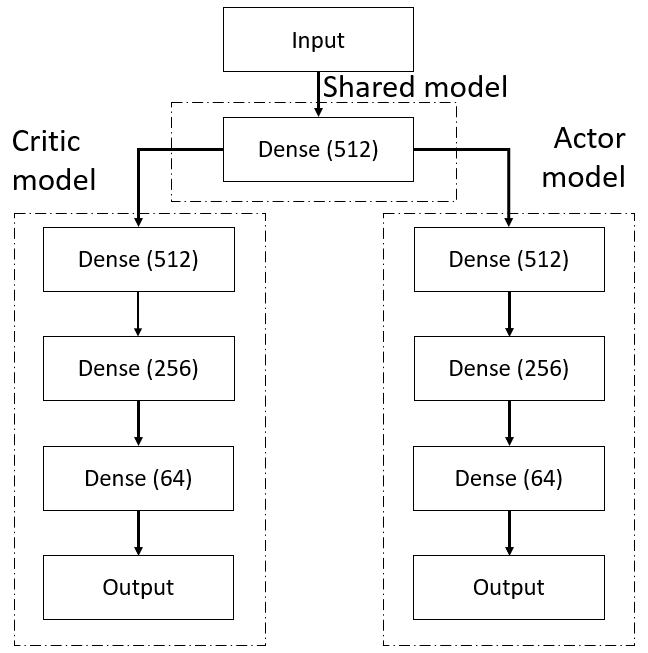
A = Dense(64, activation="relu")(A)

This is one of the primary methods we tried. But somewhere on the internet, I read that it's a good idea to have some shared layers between Actor and Critic:

# Shared Dense layers:
X = Flatten()(X_input)
X = Dense(512, activation="relu")(X)

# Critic model
V = Dense(512, activation="relu")(X)
V = Dense(256, activation="relu")(V)
V = Dense(64, activation="relu")(V)
value = Dense(1, activation=None)(V)

# Actor model
A = Dense(512, activation="relu")(X)
A = Dense(256, activation="relu")(A)
A = Dense(64, activation="relu")(A)

This means that, for example, two first neural networks should be used by both networks, and only the next (head) layers should be separated. Here is an example image:

Also, we will try to use recurrent neural networks used for time series and convolution neural networks, which are mostly used for image classification and detection.

Recurrent Networks

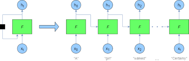
One of the apparent changes we need to test is to update our model to use a recurrent or so-called Long Short-Term Memory (LSTM) network in place of our previous Dense network. Since recurrent networks can maintain an internal state over time, it's unnecessary to use a sliding "look-back" window to capture the history of the price action. Instead, it is captured essentially by the recursive nature of the network. At each timestep, the input from the dataset is passed into the algorithm, along with the output from the last timestep. I am not going to remove it yet from my code so it won't mess us up, and we'll be able to test which of our models performs better. Also, I am pretty unfamiliar with LSTM networks, so I don't know by myself how to implement them correctly, but here is a pretty informative introduction to it.

This structure of the LSTM model allows the internal state to be maintained, which is updated every time the agent "remembers" and "forgets" specific data relationships:

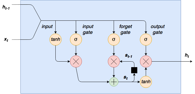
I am not going deep into LSTM, because as I said, I am not very familiar with it, but I have plans to do time series analysis and tutorial series in the future. So, this is how our model will look with LSTM shared layers:

# Shared LSTM layers:
X = LSTM(512, return_sequences=True)(X_input)
X = LSTM(256)(X)

# Critic model
V = Dense(512, activation="relu")(X)
V = Dense(256, activation="relu")(V)
V = Dense(64, activation="relu")(V)
value = Dense(1, activation=None)(V)

# Actor model
A = Dense(512, activation="relu")(X)
A = Dense(256, activation="relu")(A)
A = Dense(64, activation="relu")(A)

Convolutional Networks

CNN's have been, by far, the most commonly adopted deep learning model. Meanwhile, most of the CNN implementations in the literature were chosen to address computer vision and image analysis challenges. With successful deployments of CNN models, the model error rates keep dropping over the years while new CNN complicated architectures are invented. Nowadays, almost all computer vision researchers, one way or another, implement CNN in image classification problems.

In this paper, a study was introduced, where authors propose a novel approach that converts 1-D financial time series into a 2-D image-like data representation to be able to utilize the power of the deep convolution neural network for an algorithmic trading system. However, the authors wrote an interesting article and made quite impressive results. Their proposed CNN model trained on time-series images performed quite similar to the LSTM network - sometimes better, sometimes worse. But significant improvement is that CNN doesn't require as much computational power and time to train the model, so we'll train our agent and test it with the following model:

# Shared CNN layers:
X = Conv1D(filters=64, kernel_size=6, padding="same", activation="tanh")(X_input)
X = MaxPooling1D(pool_size=2)(X)
X = Conv1D(filters=32, kernel_size=3, padding="same", activation="tanh")(X)
X = MaxPooling1D(pool_size=2)(X)
X = Flatten()(X)

# Critic model
V = Dense(512, activation="relu")(X)
V = Dense(256, activation="relu")(V)
V = Dense(64, activation="relu")(V)
value = Dense(1, activation=None)(V)

# Actor model
A = Dense(512, activation="relu")(X)
A = Dense(256, activation="relu")(A)
A = Dense(64, activation="relu")(A)

Other minor changes

So, up to this point, we mainly talked about our reward and model improvements. But there are also other ways to make our lives easier when training and testing different models in between.

First of all, I changed how we save our model because I don't know when the model is over-fitting and what signalizes about this sign. At least right now, I decided to keep every best model. So instead of saving the best model on top of our older models, I am creating a new folder where I will save these models and use the average reward as a name for them.

I noticed that when I was testing my models, it got pretty messy, and I can't remember the best results of my model. Also, I saw that it's pretty hard to remember all the parameters we set while testing/training every new model, so I am creating a Parameters.txt file in the exact model-saving location. So I write the following parameters to a text file:

params.write(f"training start: {current_date}\n")
params.write(f"initial_balance: {initial_balance}\n")
params.write(f"training episodes: {train_episodes}\n")
params.write(f"lookback_window_size: {self.lookback_window_size}\n")
params.write(f"lr: {self.lr}\n")
params.write(f"epochs: {self.epochs}\n")
params.write(f"batch size: {self.batch_size}\n")
params.write(f"normalize_value: {normalize_value}\n")
params.write(f"model: {self.comment}\n")

So, I will now know what initial balance I started with, what look-back window I used, what learning rate was used for training, how many epochs I used for one episode, what normalization value I used. Finally, I can write what model type I use; this makes my test results much easier!

Another essential step in our testing results, it's convenient to have them in one place for comparison simplicity. So I inserted the following lines into my code:

print("average {} episodes agent net_worth: {}, orders: {}".format(test_episodes, average_net_worth/test_episodes, average_orders/test_episodes))
print("No profit episodes: {}".format(no_profit_episodes))
# save test results to test_results.txt file
with open("test_results.txt", "a+") as results:
    results.write(f'{datetime.now().strftime("%Y-%m-%d %H:%M")}, {name}, test episodes:{test_episodes}')
    results.write(f', net worth:{average_net_worth/(episode+1)}, orders per episode:{average_orders/test_episodes}')
    results.write(f', no profit episodes:{no_profit_episodes}, comment: {comment}\n')

With these results, we can compare with what average net_worth our agent traded all testing episodes, how many orders it did on average through the episode, and one of the most important metrics would be "no profit episodes" - this will show us, how many episodes we finished in the negative side through our testings. Also, there are a lot of metrics we could add, but now, it's enough for us to compare and choose the best we need. Also, this way, we'll be able to test the bulk of models at once, leave it for a night, and check results in the morning.

Also, I did minor modifications to the model save function, and now while saving our model, we will be able to log our parameters about the current saved model time step with the following function:

def save(self, name="Crypto_trader", score="", args=[]):
    # save keras model weights
    self.Actor.Actor.save_weights(f"{self.log_name}/{score}_{name}_Actor.h5")
    self.Critic.Critic.save_weights(f"{self.log_name}/{score}_{name}_Critic.h5")

    # log saved model arguments to file
    if len(args) > 0:
        with open(f"{self.log_name}/log.txt", "a+") as log:
            current_time = datetime.now().strftime('%Y-%m-%d %H:%M:%S')
            log.write(f"{current_time}, {args[0]}, {args[1]}, {args[2]}, {args[3]}, {args[4]}\n")

Training and testing

Training our models

As I already mentioned, I will train all models on the same dataset with the same parameters. I am only going to change the model type. After training, we'll be able to compare training duration, compare Tensorboard training graphs, and of course, we'll get trained models. We'll test all of these trained models on the same testing dataset, and we'll see how they perform on unseen market data! We have three different model architectures (Dense, CNN, and LSTM). Now I'll invest my time and my 1080TI GPU to make this first comparison between architectures.

So, I started training the model from the simplest Dense model with the following code lines:

if __name__ == "__main__":            
    df = pd.read_csv('./pricedata.csv')
    df = df.sort_values('Date')

    lookback_window_size = 50
    test_window = 720 # 30 days 
    train_df = df[:-test_window-lookback_window_size]
    test_df = df[-test_window-lookback_window_size:]
    
    # Create our custom Neural Networks model
    agent = CustomAgent(lookback_window_size=lookback_window_size, lr=0.00001, epochs=5, optimizer=Adam, batch_size = 32, comment="Dense")
    
    # Create and run custom training environment with following lines
    train_env = CustomEnv(train_df, lookback_window_size=lookback_window_size)
    train_agent(train_env, agent, visualize=False, train_episodes=50000, training_batch_size=500)

When the training starts, you can see that a new folder with the current date and time is created in the same folder where we can find the Parameters.txt file. If I would open this file, we can see all our current used settings in it:

training start: 2021–01–11 13:32
initial_balance: 1000
training episodes: 50000
lookback_window_size: 50
lr: 1e-05
epochs: 5
batch size: 32
normalize_value: 40000
model: Dense
training end: 2021–01–11 18:20

As you can see, in this file, we saved all the parameters that we used to train our model; we can even see how long it took to train my model. This helps later when we'll be trying to find the best-optimized model or train different models manually, usually because it takes some time. As you can see, it is easy to forget what parameters we used.

Also, we can see that the log.txt file was created, here is saved all saved model statistics at that time. These might help to find the best model we trained that is not overfitting.

All the models our agent saves are located in the same directory. So, when we are testing them, we'll need to specify our model's correct directory and name.

Bellow is my snip from Tensorboard while training Dense (Orange color) and CNN (Blue color) networks for 50k training steps. It's sad, but by my mistake, I removed the LSTM training graph. It took me too long that I could train it again. I will do that in the coming tutorials when our model will be a little better:

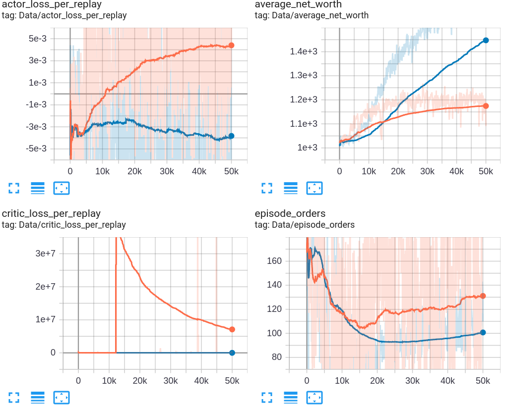
Right now, let's compare Dense and CNN models and how they trained. First, let's look at the average_net_worth graph. As we can see, our CNN model learned to get much higher rewards in time, but we shouldn't trust these results blindly. I think that our CNN might be overfitting. First of all, it looks pretty suspicious to me how our critic network was training and how this critic_loss_per_replay graph looks for our CNN. Numbers are a hundred times bigger than while training the Dense model.

Second, while looking at our actor_loss_per_replay graph, we can see that we might see quite a beautiful curve while training the Dense model. We can see that this curve has been coming in an up direction since around the 20k episode. But while seeing the CNN training actor loss curve on the same graph gives some training instability. But ok, this is my preliminary view; we'll test both models, that one on the curve top and the best model by average net worth.

Also, it's pretty interesting to see the average episode orders graph because we added a punish value into our reward strategy it's pretty logical that our model tries to avoid this punishment and learn to do as many orders as possible. But instead of doing orders every step, it discovered that sometimes it's better to be punished and wait for better order conditions where it could get a positive reward!

Testing our models

As you already know, we trained three different models (Dense, CNN, LSTM) for 50k training steps. We can test all of them at once with the following code:

if __name__ == "__main__":            
    df = pd.read_csv('./pricedata.csv')
    df = df.sort_values('Date')

    lookback_window_size = 50
    test_window = 720 # 30 days 
    train_df = df[:-test_window-lookback_window_size]
    test_df = df[-test_window-lookback_window_size:]

    agent = CustomAgent(lookback_window_size=lookback_window_size, lr=0.00001, epochs=1, optimizer=Adam, batch_size = 32, model="Dense")
    test_env = CustomEnv(test_df, lookback_window_size=lookback_window_size, Show_reward=False)
    test_agent(test_env, agent, visualize=False, test_episodes=1000, folder="2021_01_11_13_32_Crypto_trader", name="1277.39_Crypto_trader", comment="")

    agent = CustomAgent(lookback_window_size=lookback_window_size, lr=0.00001, epochs=1, optimizer=Adam, batch_size = 32, model="CNN")
    test_env = CustomEnv(test_df, lookback_window_size=lookback_window_size, Show_reward=False)
    test_agent(test_env, agent, visualize=False, test_episodes=1000, folder="2021_01_11_23_48_Crypto_trader", name="1772.66_Crypto_trader", comment="")
    test_agent(test_env, agent, visualize=False, test_episodes=1000, folder="2021_01_11_23_48_Crypto_trader", name="1377.86_Crypto_trader", comment="")

    agent = CustomAgent(lookback_window_size=lookback_window_size, lr=0.00001, epochs=1, optimizer=Adam, batch_size = 128, model="LSTM")
    test_env = CustomEnv(test_df, lookback_window_size=lookback_window_size, Show_reward=False)
    test_agent(test_env, agent, visualize=False, test_episodes=1000, folder="2021_01_11_23_43_Crypto_trader", name="1076.27_Crypto_trader", comment="")

Our most straightforward dense network for 1000 episodes scored 1043.40$ on average net worth in my previous tutorial. That's the score we want to beat.

Dense

First, I trained and tested the Dense network and received the following results:

Model name: 1277.39_Crypto_trader
net worth: 1054.483903083776
orders per episode: 140.566
no profit episodes: 14

As you can see in the previous tutorial, we didn't measure how many orders per episode our model does and how many orders finished in negative net worth through 1000 episodes. Anyway, we can see that our Dense current model with the new reward strategy did a little better! But this metric is not that important as the new "no profit episodes" metric because it's better to have lower profit but be sure that our model won't lose our money. So it's best to evaluate "net worth" together with the "no profit episodes" metric.

CNN

Next, I trained and tested the Convolution Neural Networks (CNN) model, you may find many articles about CNN in time series, but this is not the topic to talk about. So I'll take the saved model with the best average reward, and let's see the results:

Model name: 1772.66_Crypto_trader
net worth: 1008.5786807732876
orders per episode: 134.177
no profit episodes: 341

As we can see, our model doesn't perform as well as it was performing while training. We have some overfitting with it. Results are terrible 34% of orders had a negative ending balance, and profit was even worse than the random model. So I decided to test another CNN model that has less overfitting relying on the Tensorboard graph:

Model name: 1124.03_Crypto_trader
net worth: 1034.3430652376387
orders per episode: 70.152
no profit episodes: 55

As we can see, this model performed much better than training it up to the end, but still, our most straightforward Dense network wins against it with a testing dataset.

LSTM

Finally, I thought that let's try to train the LSTM Network. Moreover, the dataset is created for time series data; it should perform well:

Model name: 1076.27_Crypto_trader
net worth: 1027.3897665208062
orders per episode: 323.233
no profit episodes: 303

To train the LSTM network took around three times longer than the Dense and CNN networks, so I was despondent when I wasted so much time and received awful results. I thought that I was going to do something interesting, but now we have what we have.

Conclusion:

I decided to stop my article because it took me too long to do these written experiments and compare them. But I am glad that I was able to improve my Dense network profitability with a new strategy.

I won't rush to say that it is inappropriate to use CNN's and LSTM's to predict time series marked data. In my opinion, we used too little training data that our model could adequately learn all market features.

I won't give up so quickly. I still think that our Neural Networks can beat the market, but he needs more data. So I have plans shortly to write at least two more tutorials:

1. We'll try to implement indicators to our market data, so our model will have more features to learn from;
2. It's pretty obvious that we are using too little training data to train our model, so we'll write some script to download more historical data from the internet;
3. We'll write a copy of our custom trading environment that we could use in parallel, using multiprocessing to run multiple training environments to speed up the training process.

Thanks for reading! There is still a lot of work to do. Subscribe and like my video on YouTube, share this tutorial, and you'll be notified when another tutorial will see the daylight! As always, all the code given in this tutorial can be found on my GitHub page and is free to use! See you in the next part.

All of these tutorials are for educational purposes and should not be taken as trading advice. It would be best to not trade based on any algorithms or strategies defined in this, previous, or future tutorials, as you are likely to lose your investment.