To be a state-of-the-art model, YOLOv4 needs to be at the leading edge of deep learning. YOLOv4 authors have worked on techniques to improve the accuracy of the model while training and in post-processing.

These techniques are called bag-of-freebies and bag-of-specials. In my previous tutorial, we mostly covered the YOLOv4 backbone, the neck, and part of bag-of-specials (BoS) for the detector. So, in this part, we will continue bag-of-specials (BoS) and cover bag-of-freebies (BoF).

Here's the complete list from the paper:

• BoS for backbone: Mish activation, Multi-input weighted residual connections (MiWRC), cross-stage partial connections (Talked in the previous tutorial);
• BoS for detector: Mish activation, SPP-block, SAM-block, PAN path-aggregation block, DIoU-NMS;
• BoF for backbone: CutMix and Mosaic data augmentation, DropBlock regularization, Class label smoothing;
• BoF for detector: CIoU-loss, CmBN, Self-Adversarial Training, Eliminate grid sensitivity, Using multiple anchors for single ground truth, Cosine annealing scheduler, Optimal hyperparameters, and Random training shapes.

Bag of Specials (BoS) for backbone

Mish activation:

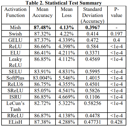
If you look at the YOLOv4 backbone, you may see that it uses the Mish activation function in the backbone. Mish is another activation function with a close similarity to ReLU. As claimed by the paper, Mish can outperform them in many deep networks across different datasets:

Mish is a novel smooth and non-monotonic neural activation function which can be defined as:

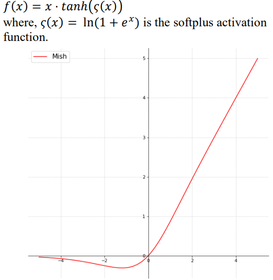It turns out that this activation function shows encouraging results. For example, using a Squeeze Excite Network with Mish (on CIFAR-100 dataset) increased Top-1 test accuracy by 0.494% and 1.671% compared to the same network with Swish and ReLU, respectively.

Multi-input weighted residual connections (MiWRC):

In recent years, researchers have paid a lot of attention to feature maps and what will be fed into the CNN layer. Almost all current object detection models start to break away from the tradition that only the previous layer is used for the next layer.

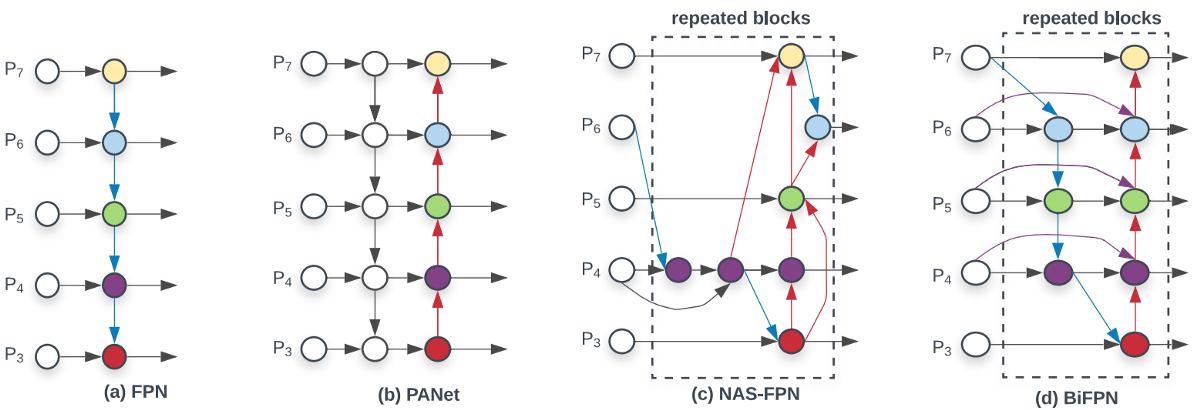
How layers are connected in object detection becomes more and more critical now. I already mentioned that in my previous tutorial while talking about FPN and PAN. Now I will show the diagram (d) below that shows another neck design called BiFPN that has better accuracy and efficiency trade-offs according to the BiFPN paper:

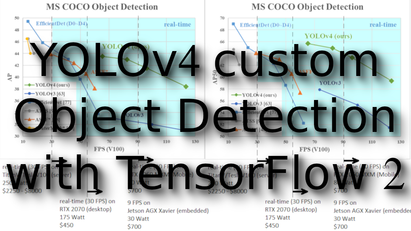
In the YOLOv4 paper, the authors compare its performance with the EfficientDet, which is considered one of the state-of-the-art technology by YOLOv4. As shown below, EfficientDet uses the EfficientNet as the backbone feature extractor and BiFPN as the neck:

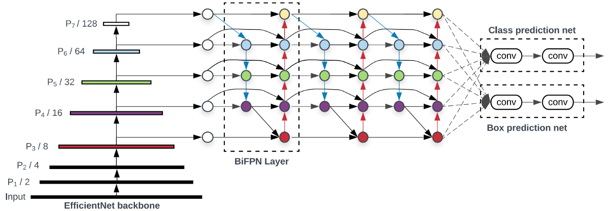
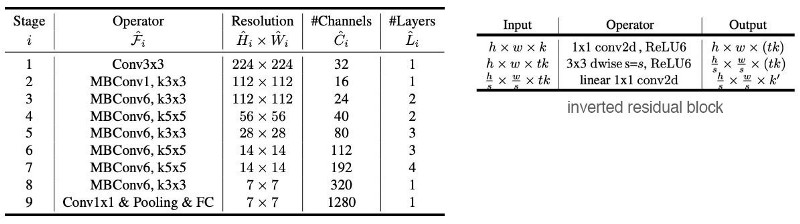
As a reference, the diagram below is the architecture for the EfficientNet, which builds on the MBConv layers that compose of the inverted residual block:

The essential advantage of this is that it requires much lower computation resources than the traditional convolution layer.

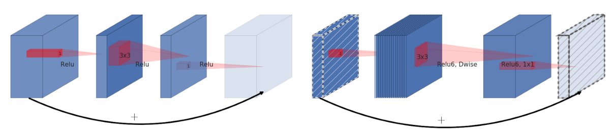
In many ML and DL problems, we learn a low-dimensional representation of the input. We extract the core information of the data by creating an "information" bottleneck. That forces us to discover the most crucial information, which is the core principle of learning. Following this principle, an Inverted residual block takes a low-dimensional representation as input and manipulates it with convolution (linear operation) and non-linear operations. But there is a major issue with the non-linear parts like ReLU. Non-linear operations stretch or compress regions un-proportionally. In such compression, inputs may map to the same regions/points. For example, ReLU may collapse the channel in this low-dimensional space and inevitably lose information.

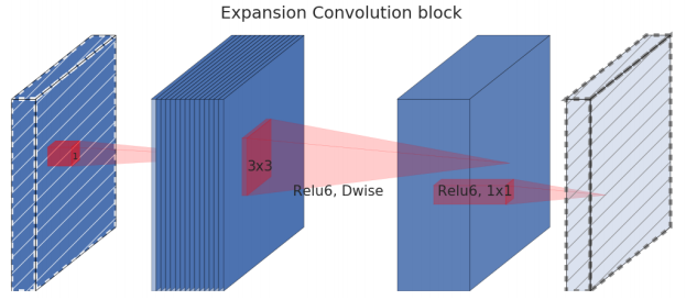
To address that, we can temporarily expand the dimension (the number of channels). We hope that we have lots of channels now, and information may still be preserved in some channels after the non-linear operations. Here is the detail of an inverted residual block:

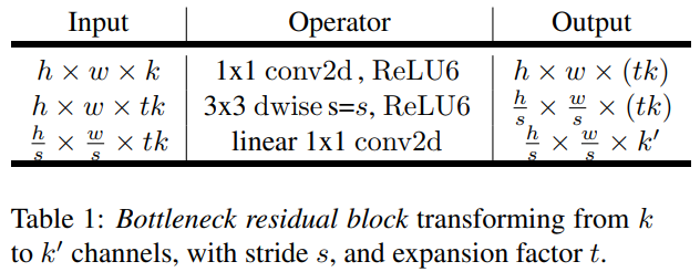
As shown above, the low-dimensional representation is first expanded to tk channels. Then, it is filtered with lightweight 3x3 depthwise convolution. Features are then subsequently reduced back to a low-dimensional at the end of the module. Non-linear operations are added when it remains in the higher-dimensional space:

A residual connection is added from the beginning to the end of the module. The diagram on the left is the traditional residual block, and the right is the described inverted residual block:

The main contribution of EfficientDet on the YOLOv4 paper is the Multi-input weighted residual connections. The EfficientDet paper observes that different input features are at different resolutions and unequally contribute to the output feature. But I already mentioned in my previous tutorial that we add those features equally instead of weighting input features differently.

Bag of Specials (BoS) for detector

I already talked about Mish activation above, and I covered SPP, SAM, and PAN path-aggregation blocks in my previous tutorial, so I don't want to repeat myself. So, I will take a brief look at DIoU-NMS.

DIoU-NMS:

We already should have heard about NMS and that they filter out other boundary boxes that predict the same object and retain one with the highest confidence:

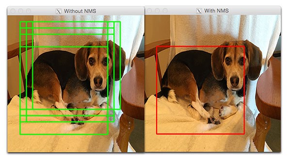The DIoU (will cover it later together with CIoU-loss) is employed as a factor in non-maximum suppression (NMS). When suppressing redundant boxes, this method takes IoU and the distance between the central points of two bounding boxes. This makes it more robust for the cases with occlusions.

Bag of Freebies (BoS) for backbone

CutMix data augmentation:

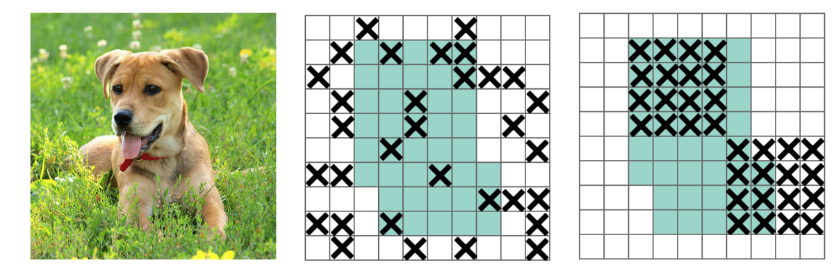
The best way to explain CutMix data augmentation is with the following image from CutMix paper:

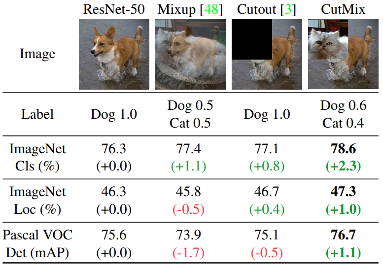
From the image above, we can see that Cutout data augmentation removes a region of an image. This forces the model not to be overconfident on specific features in making classifications. However, a portion of the image is filled with useless information, and this is a waste. In the CutMix, a part of an image is cut-and-paste over another image. The ground truth labels are readjusted proportionally to the area of the patches, e.g. 0.6 like a dog and 0.4 like a cat.

Conceptually, CutMix has a broader view of what an object may compose. The cutout area forces the model to learn object classification with different sets of features. This avoids overconfidence. Since that area is replaced with another image, the amount of information in the image and the training efficiency will not be significantly impacted. While reading YOLOv4, I first time faced such a technique that was quite interesting to me.

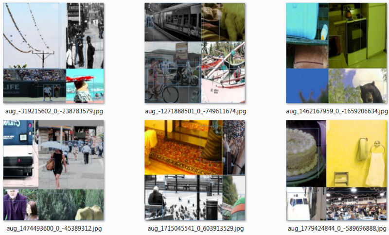
Mosaic data augmentation:

Another technique is a Mosaic data augmentation method that combines four training images into one for training (instead of 2 in CutMix). This enhances the detection of objects outside their everyday context. In addition, each mini-batch contains a large variant of image (4×) and, therefore, reduces the need for large mini-batch sizes in estimating the mean and the variance:

DropBlock regularization:

We used to know what is Dropout, but in YOLOv4, authors applied fully-connected layer dropoff to force the model to learn from a variety of features instead of being too confident on a few. However, this may not work for convolution layers. Neighboring positions are highly correlated. So even some of the pixels are dropped (the middle diagram below), the spatial information remains detectable. DropBlock regularization builds on a similar concept that works on convolution layers:

So, instead of dropping individual pixels, a block of block_size x block_size of pixels is dropped.

Class label smoothing:

In machine learning or deep learning, we usually use many regularization techniques, such as L1, L2, Dropout, etc., to prevent our model from overfitting. In classification problems, sometimes our model would learn to predict the training examples exceptionally confidently. This is not good for generalization.

Label smoothing adjusts the target upper bound of the prediction to a lower value, say 0.9. And it will use this value instead of 1.0 in calculating the loss. This concept mitigates overfitting:

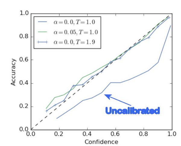So, label smoothing is a regularization technique for classification problems to prevent the model from predicting the labels too confidently during training and generalizing poorly. More about label smoothing you can read on this paper.

Bag of Freebies (BoS) for detector

CIoU-loss:

A loss function tells us how to adjust weights to reduce total cost. So in situations where we make wrong predictions, we expect it to give us direction on where to move. But this is not happening when we use IoU when the ground truth box and the prediction do not overlap. Let's consider two predictions (both do not overlap with the ground truth). In this situation, the IoU loss function cannot tell which prognosis is better, even if one may be closer to the ground truth than the other:

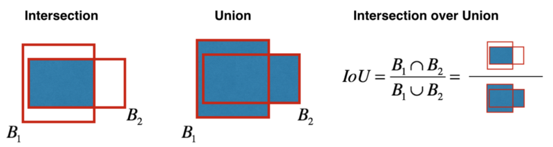Here is another example from the IoU paper:

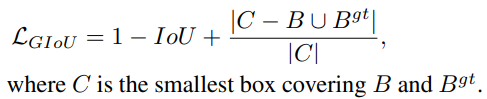
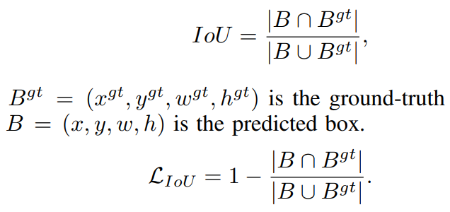Generalized IoU (GIoU) fixes the above problem by refining the loss as:

But this loss function tends to expand the prediction boundary box first until it is overlapped with the ground truth. Then it shrinks to increase IoU. This process requires more iterations than theoretically needed. To solve this, Distance-IoU Loss (DIoU) was introduced:

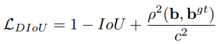
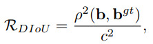Where b and bᵍᵗ denote the central points of B and Bᵍᵗ, ρ is the Euclidean distance, and c is the diagonal length of the smallest enclosing box covering the two boxes. And then the DIoU loss function can be defined as:

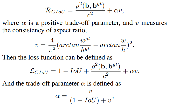
Finally, Complete IoU Loss (CIoU) was introduced to:

• Increase the overlapping area of the ground truth box and the predicted box;
• Minimize their central point distance;
• Maintain the consistency of the boxes aspect ratio.

This is the last definition from the paper:

The CmBN (Cross mini-Batch Normalization):

The original Batch normalization collects the samples of mean and variance within a mini-batch to whiten the layer input. However, as weights change in each iteration, the statistics collected under those weights may become inaccurate under the new weight. However, if the mini-batch size is small, these estimations will be noisy. One solution is to estimate them among many mini-batches. In Cross-Iteration Batch Normalization (CBM), it estimates those statistics from k previous iterations with the following adjustment:

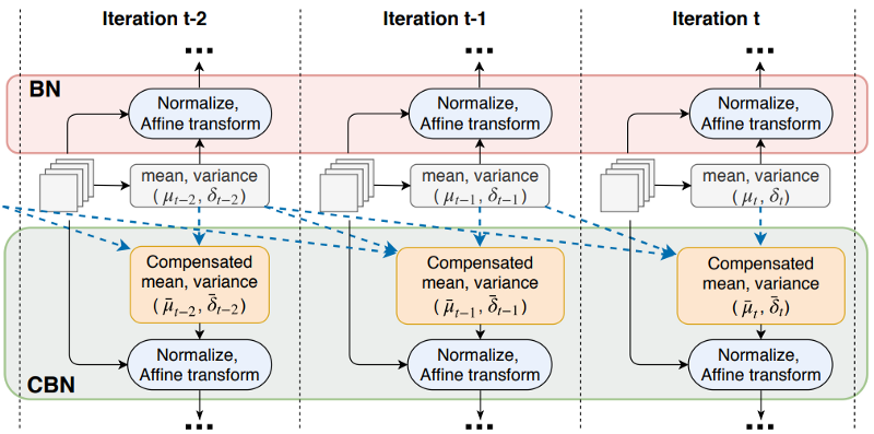
The CmBN is a modified representation of CBN, which assumes that a batch contains four mini-batches.

CmBN (Cross mini-Batch Normalization):

Self-Adversarial Training (SAT) is a data augmentation technique. First, it performs a forward pass on a training sample. Traditionally, in backpropagation, we adjust the model weights to improve the detector detecting objects in a specific image. While in SAT, we change the image such that it can degrade the detector performance the most. i.e., it creates an adversarial attack targeted for the current model even though the new image may look visually the same, as in the following example:

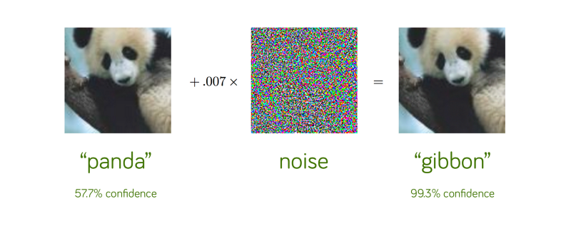Then the model is trained with this new image with the original boundary box and class label. This helps to generalize the model and to reduce overfitting.

Eliminate grid sensitivity:

I couldn't find much information about this step, but it's known that old YOLO models do not do an excellent job of making predictions right around the boundaries of anchor box regions. So, it is helpful to define box coordinates slightly differently to avoid this problem. So, this technique was presented in YOLOv4. We know that the boundary box is computed as follows:

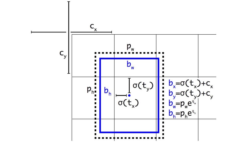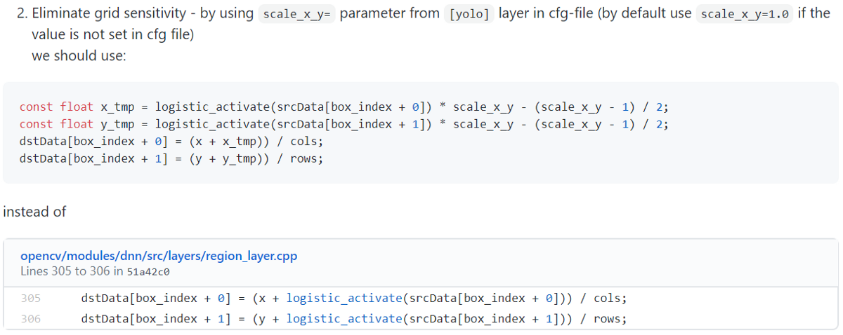
For the cases bₓ = cₓ and bₓ = cₓ+1, we need tₓ to have a substantial negative and positive value, respectively. But we can multiply σ with a scaling factor (>1.0) to make it easier. Here is the source for proposed changes:

Cosine annealing scheduler:

I am already using this technique from my YOLOv3 implementation, but let's cover it again. The cosine schedule adjusts the learning rate according to a cosine function. It starts by reducing the significant learning rate slowly. Then it reduces the learning rate quickly halfway and finally ends up with a slight slope in lowering the learning rate:

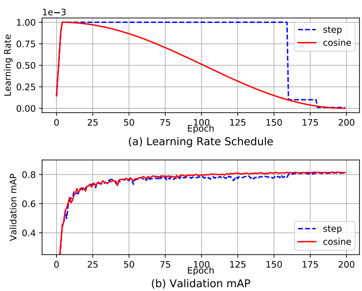
The diagram above shows how the learning rate is decay (learning rate warmup is also applied) and its impact on the mAP. It may not be pronounced, but this method has more constant progress rather than plateau for a long while before making progress again.

Optimal hyperparameters:

I can't find much information related to this topic, but as I understood, the authors offered to select hyperparameters by using genetic algorithms. For example, we choose 100 sets of hyperparameters randomly. Then, we use them for training 100 models. Later, we select the top 10 performed models. For each selected model, then it's created ten slightly mutated hyperparameters according to their original. And after that, we retrain the models with the new hyperparameters and choose the best models again. As we keep the iterations, we should find the best set of hyperparameters. Alternatively, we can start with the default hyperparameters, and then we start the mutations. But anyway, this method takes an enormous amount of time and resources.

Random training shapes:

I can't find much information about this part, but it's known that most single-stage object detectors are trained with a fixed input image shape. To improve generalization, the authors offered to train the model with different image sizes. (Multi-Scale Training in YOLO).

Conclusion:

So, in summary, the authors offered a state-of-the-art detector that is faster in terms of Frames per Second (FPS) and more accurate on MS COCO AP50:::95 and AP50 than all available alternative detectors. Also, it is nice that YOLOv4 can be trained and used on a conventional GPU with 8–16GB VRAM, which is broadly available. I must say a big well done to the authors for having verified many features and selected them for use, such as improving the accuracy of both the classifier and the detector. These features can be used as best-practice for future studies and developments. I also implemented YOLOv4 architecture on top of my YOLOv3 implementation to run the model within TensorFlow 2. But sadly, I didn't have time to implement all these Bag-Of-Freebies to improve the training process. Maybe later I'll find time to do that, but now I leave it as it is. So, you can clone my GitHub repository and test it out! How to train it written in the readme file.