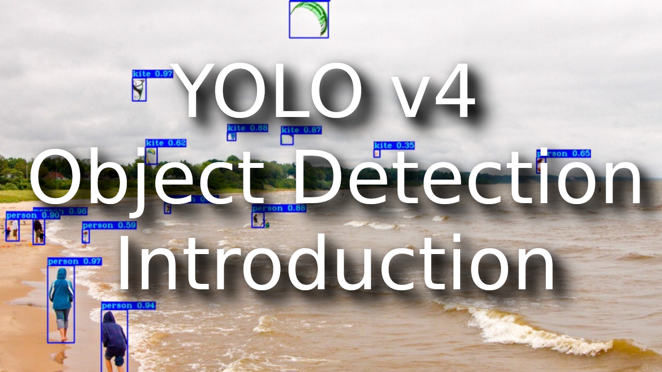
YOLO stands for You Only Look Once. It's an object detection model used in deep learning use cases. In this article, I will not talk about the history of the previous YOLO versions or the background of how it works. If you are interested in details on how it works, you can check my previous articles about it.
No one in the research community expected a YOLOv4 to be released…
Why? Joseph Redmon, the original author, had announced that he would stop doing computer vision research because of military and ethical issues.
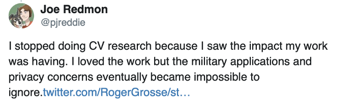 But someone had continued the hard work… and it was Alexey Bochkovskiy!
YOLO belongs to the family of One-Stage Detectors (You only look once - one-stage detection). One-stage detection (also referred to as one-shot detection) is that you only look at the image once. If we needed to answer what does it mean in fewer sentences, it would sound the following:
- It is a sliding window and classification approach, where you look at the image and classify it for every window;
- In a region proposal network, you look at the image in two steps - the first to identify regions where there might be objects and the next to specify it.
YOLOv4
In this article, we'll try to understand why the release of YOLOv4 spread through the internet in just a few days, why it's called a super-network that can, once again, change the world, same as YOLOv3 did.
Most people in the field today are used to YOLOv3, which already produces excellent results. But now, YOLOv4 has improved again in terms of accuracy (average precision) and speed (FPS) - the two metrics we generally use to qualify an object detection algorithm:
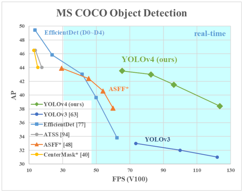
As shown above, YOLOv4 claims to have state-of-the-art accuracy while maintaining a high processing frame rate. It achieves an accuracy of 43.5% AP for the MS COCO with an approximately 65 FPS inference speed on the Tesla V100. In object detection, high accuracy is not the only holy grail anymore. We want the model to run smoothly in the edge devices. Processing video input in real-time with low-cost hardware becomes essential also.
Before diving into the details in this article, I recommend you to read the YOLOv4 paper.
What changed in YOLOv4 (Bag-of-Freebie and Bag-of-Specials):
- Bag-of-Freebie (This tutorial part) - Specific improvements made in the training process that have no impact on inference speed and increase accuracy (like data augmentation, class imbalance, cost function, soft labeling, etc.);
- Bag-Of-Specials (Second tutorial part) - Improving the network slightly impacts the inference time with a good performance return. These improvements include increasing the receptive field, using attention, feature integration like skip-connections, and post-processing like non-maximum suppression.
There is so much to cover about YOLOv4 that I decided to write this article in two parts. In this article, I will discuss how the feature extractor and the neck are designed. Then I'll give you the code of YOLOv4 implementation to run the pre-trained model.
The second part will be about the training process.
YOLOv4 Architecture
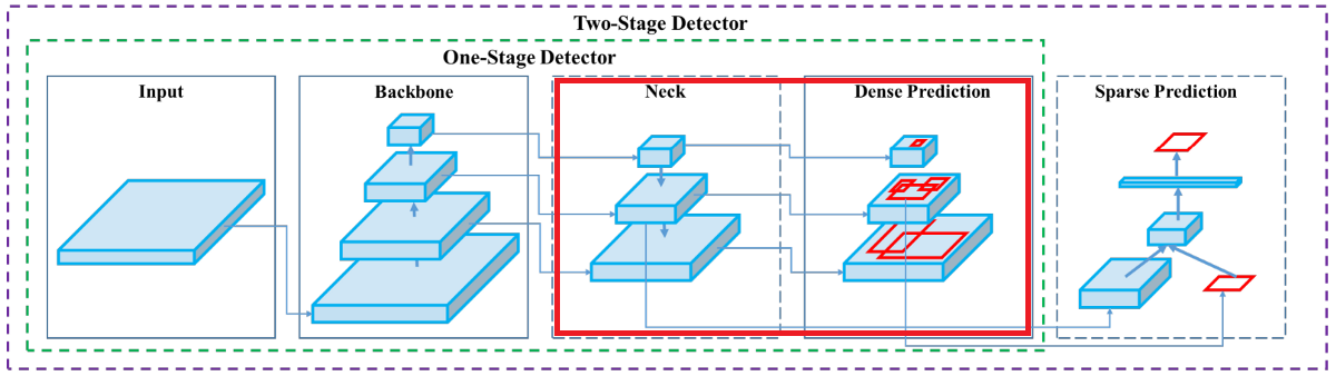
Following architecture is provided in the paper:
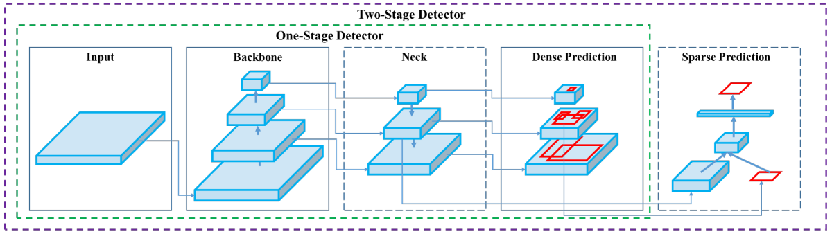
We have four parent blocks after the input image:
- Backbone (Dense Block & DenseNet, CSP, CSPDarknet53);
- Neck (FPN, SPP);
- Head (Dense Prediction) - used in one-stage-detection algorithms such as YOLO, SSD, etc.;
- Sparse Prediction - used in two-stage-detection algorithms such as Faster-R-CNN, etc. (not in YOLOv4).
Backbone
Backbone here refers to the feature-extraction architecture. You should know it by different names if you're used to YOLO, such as YOLO Tiny or Darknet53. The difference between these is the backbone.
- YOLO-Tiny has only nine convolutional layers, so it's less accurate but faster, less resource-hungry, and better suited for mobile and embedded projects;
- Darknet53 has 53 convolutional layers, so it's more accurate but slower.
Looking at the YOLOv4 paper, you'll notice that the backbone used isn't Darknet53 but CSPDarknet53. These letters are not here to look nice - they mean something, so we'll try to understand this.
Backbone is one of the ways where we can improve accuracy. We can expand this concept further with highly interconnected layers. We can design a deeper network to extend the receptive field and increase model complexity. And to ease the training difficulty, skip-connections can be applied.
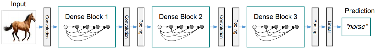
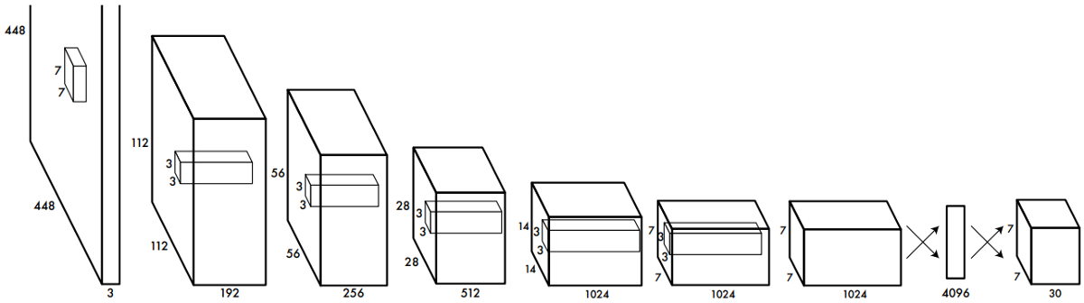
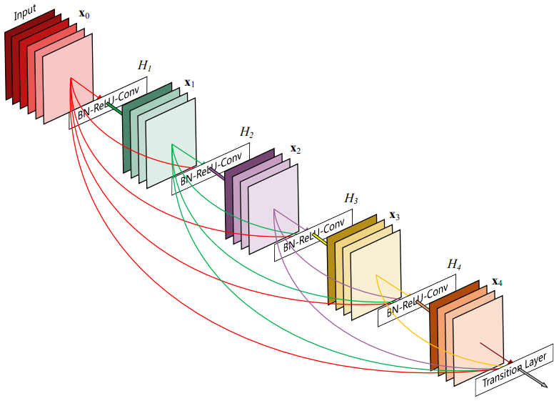
A Dense Block in the YOLOv4 backbone contains multiple convolution layers, with each layer Hi is composed of batch normalization, ReLU, and then convolution. Instead of using the output of the last layer only, Hi takes the output of all previous layers and the original as its input. i.e., x₀, x₁, ..., and xᵢ₋₁. Each Hi below outputs four feature maps. Therefore, at each layer, the number of feature maps is increased by four - the growth rate:

Then a DenseNet can be formed by composing multiple Dense Blocks with a transition layer in between that composed of convolution and pooling:
CSP stands for Cross-Stage-Partial connections. The idea here is to separate the input feature maps of the DenseBlock into two parts, one that will go through a block of convolutions and one that won't. Then, we aggregate the results. Here's an example with DenseNet:
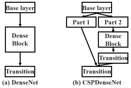
This new design reduces the computational complexity by separating the input into two parts - with only one going through the Dense Block.
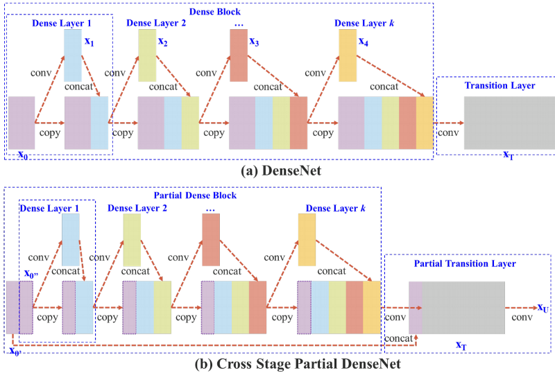
Above is an illustration of DenseNet and proposed Cross-Stage-Partial DenseNet (CSPDenseNet). CSPNet separates the feature map of the base layer into two-part. One part will go through a dense block and a transition layer. The second part will be combined with a transmitted feature map to the next stage.
CSPDarknet53 implementation looks following in my GitHub code:
def residual_block(input_layer, input_channel, filter_num1, filter_num2, activate_type='leaky'):
    short_cut = input_layer
    conv = convolutional(input_layer, filters_shape=(1, 1, input_channel, filter_num1), activate_type=activate_type)
    conv = convolutional(conv       , filters_shape=(3, 3, filter_num1,   filter_num2), activate_type=activate_type)

    residual_output = short_cut + conv
    return residual_output

def cspdarknet53(input_data):
    input_data = convolutional(input_data, (3, 3,  3,  32), activate_type="mish")
    input_data = convolutional(input_data, (3, 3, 32,  64), downsample=True, activate_type="mish")

    route = input_data
    route = convolutional(route, (1, 1, 64, 64), activate_type="mish")
    input_data = convolutional(input_data, (1, 1, 64, 64), activate_type="mish")
    for i in range(1):
        input_data = residual_block(input_data,  64,  32, 64, activate_type="mish")
    input_data = convolutional(input_data, (1, 1, 64, 64), activate_type="mish")

    input_data = tf.concat([input_data, route], axis=-1)
    input_data = convolutional(input_data, (1, 1, 128, 64), activate_type="mish")
    input_data = convolutional(input_data, (3, 3, 64, 128), downsample=True, activate_type="mish")
    route = input_data
    route = convolutional(route, (1, 1, 128, 64), activate_type="mish")
    input_data = convolutional(input_data, (1, 1, 128, 64), activate_type="mish")
    for i in range(2):
        input_data = residual_block(input_data, 64,  64, 64, activate_type="mish")
    input_data = convolutional(input_data, (1, 1, 64, 64), activate_type="mish")
    input_data = tf.concat([input_data, route], axis=-1)

    input_data = convolutional(input_data, (1, 1, 128, 128), activate_type="mish")
    input_data = convolutional(input_data, (3, 3, 128, 256), downsample=True, activate_type="mish")
    route = input_data
    route = convolutional(route, (1, 1, 256, 128), activate_type="mish")
    input_data = convolutional(input_data, (1, 1, 256, 128), activate_type="mish")
    for i in range(8):
        input_data = residual_block(input_data, 128, 128, 128, activate_type="mish")
    input_data = convolutional(input_data, (1, 1, 128, 128), activate_type="mish")
    input_data = tf.concat([input_data, route], axis=-1)

    input_data = convolutional(input_data, (1, 1, 256, 256), activate_type="mish")
    route_1 = input_data
    input_data = convolutional(input_data, (3, 3, 256, 512), downsample=True, activate_type="mish")
    route = input_data
    route = convolutional(route, (1, 1, 512, 256), activate_type="mish")
    input_data = convolutional(input_data, (1, 1, 512, 256), activate_type="mish")
    for i in range(8):
        input_data = residual_block(input_data, 256, 256, 256, activate_type="mish")
    input_data = convolutional(input_data, (1, 1, 256, 256), activate_type="mish")
    input_data = tf.concat([input_data, route], axis=-1)

    input_data = convolutional(input_data, (1, 1, 512, 512), activate_type="mish")
    route_2 = input_data
    input_data = convolutional(input_data, (3, 3, 512, 1024), downsample=True, activate_type="mish")
    route = input_data
    route = convolutional(route, (1, 1, 1024, 512), activate_type="mish")
    input_data = convolutional(input_data, (1, 1, 1024, 512), activate_type="mish")
    for i in range(4):
        input_data = residual_block(input_data, 512, 512, 512, activate_type="mish")
    input_data = convolutional(input_data, (1, 1, 512, 512), activate_type="mish")
    input_data = tf.concat([input_data, route], axis=-1)

    input_data = convolutional(input_data, (1, 1, 1024, 1024), activate_type="mish")
    input_data = convolutional(input_data, (1, 1, 1024, 512))
    input_data = convolutional(input_data, (3, 3, 512, 1024))
    input_data = convolutional(input_data, (1, 1, 1024, 512))

    input_data = tf.concat([tf.nn.max_pool(input_data, ksize=13, padding='SAME', strides=1), tf.nn.max_pool(input_data, ksize=9, padding='SAME', strides=1)
                            , tf.nn.max_pool(input_data, ksize=5, padding='SAME', strides=1), input_data], axis=-1)
    input_data = convolutional(input_data, (1, 1, 2048, 512))
    input_data = convolutional(input_data, (3, 3, 512, 1024))
    input_data = convolutional(input_data, (1, 1, 1024, 512))

    return route_1, route_2, input_data
Neck
The purpose of the neck block is to add extra layers between the backbone and the head (dense prediction block). You can see in the bellow image that different feature maps from the other layers are used:
In the early days of convolutional neural networks, everything was very linear. Networks were evolving in more recent versions; middle blocks, skip connections, and data aggregations appeared between layers. So, to enrich the information that feeds into the head, neighboring feature maps from the bottom-up and top-down streams are added together element-wise or concatenated before providing into the head. Therefore, the head's input will contain spatial rich information from the bottom-up stream and the semantic rich data from the top-down stream. This part of the system is called a neck. Let's get more details on this design.
Feature Pyramid Networks (FPN)
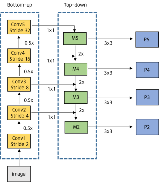
Here's a popular technique called FPN (Feature Pyramid Network), making object detection predictions at different scale levels:
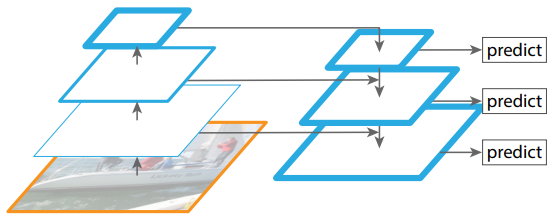
While making predictions for a particular scale, FPN upsamples (2×) the previous top-down stream and adds it with the bottom-up stream's neighboring layer (see the diagram below). The result is passed into a 3×3 convolution filter to reduce upsampling artifacts and create the feature maps P4 below for the head. In YOLOv4, the FPN concept is gradually implemented/replaced with the modified SAM, PAN, and SPP. So, let's get into them!
Spatial Attention Module (SAM)
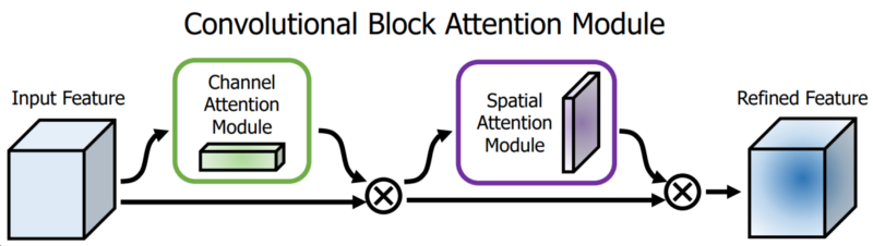
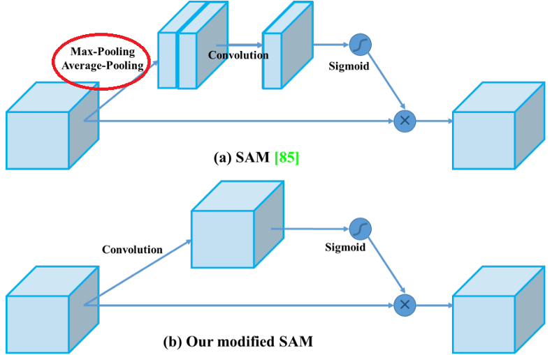
Attention mechanisms have been widely adopted in deep learning, and especially in recurrent neural network designs. The first technique used is the Spatial Attention Module (SAM). In SAM, full pool and average pool are applied separately to input feature maps to create two sets of feature maps. The results are fed into a convolution layer followed by a sigmoid function to make spatial attention:
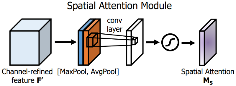
This above spatial attention module is applied to the input feature to output the refined feature maps:
But differently from the original SAM implementation, in YOLOv4, a modified SAM is used without applying the maximum and average pooling:
Path Aggregation Network (PAN)
Another technique used is a modified version of the PANet (Path Aggregation Network). The idea is again to aggregate information to get higher accuracy.
So, in early Deep Learning, the model design is relatively simple (image below). Each layer takes input from the previous layer. The early layers extract localized texture and pattern information to build up the semantic information needed in the later layers. However, as we progress to the right, localized information needed to fine-tune the prediction may be lost.
In later, deep learning was evolving, and the interconnectivity among layers was getting more and more complex. In DenseNet, it goes to the extreme. Each layer is connected with all previous layers:
In Feature Pyramid Network, information is combined from neighboring layers in the bottom-up and top-down stream:
The flow of information among Bottom-up and Top-down layers becomes another critical decision in the model design.
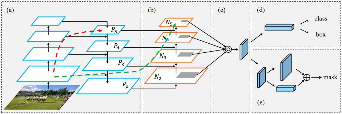
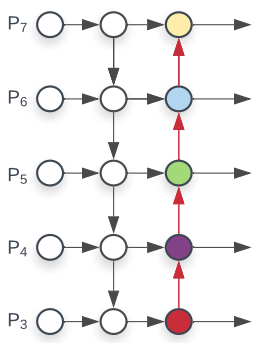
In the image below taken from Path Aggregation Network (PAN) paper, a bottom-up path (b) is augmented to make low-layer information easier to propagate to the top. In FPN, the localized spatial information travels upward in the red arrow. It is not clearly demonstrated in the image, but the red path goes through about 100+ layers. PAN introduced a short-cut path (the green path) which only takes about ten layers to go to the top N₅ layer. These short-circuit concepts make fine-grain localized information available to top layers.
Neck design (b) in EfficientDet paper is visualized as the following:
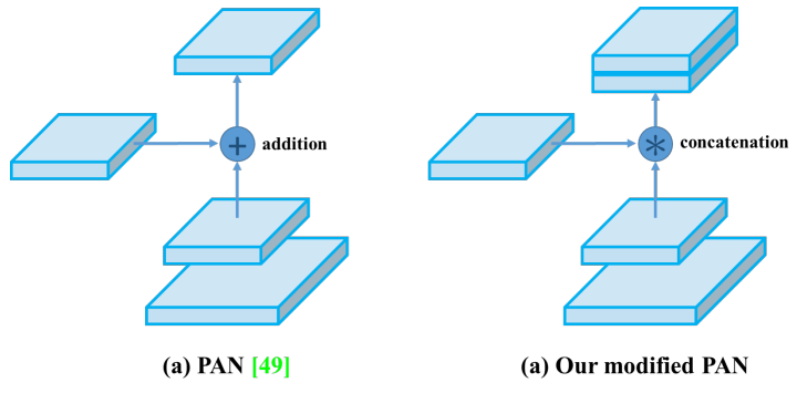
But in YOLOv4, instead of adding neighbor layers together, features maps are concatenated together:
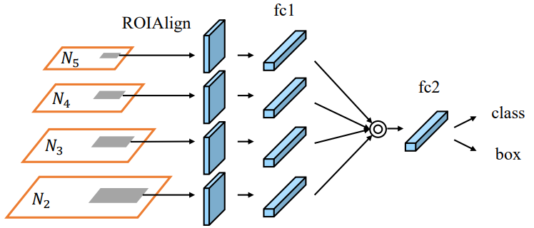
In Feature Pyramid Networks, objects are detected separately and independently at different scale levels. This may produce duplicated predictions and not utilize information from other feature maps. PAN fuses the data from all layers first using element-wise max operation:
Spatial pyramid pooling layer (SPP)
Finally, Spatial Pyramid Pooling (SPP), used in R-CNN networks and numerous other algorithms, is used here.
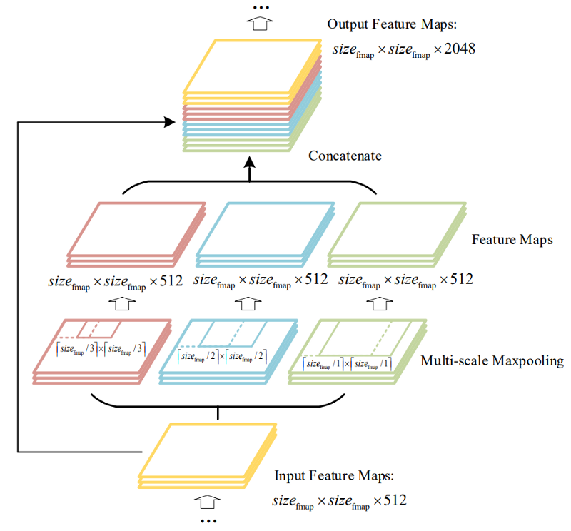
In YOLOv4, the modified SPP is used to retain the output spatial dimension. A maximum pool is applied to a sliding kernel of size say, 1x1, 5x5, 9x9, 13x13. The spatial dimension is preserved. The features maps from different kernel sizes are then concatenated together as output:
And the diagram below demonstrates how modified SPP is integrated into YOLOv4:

It's pretty hard to understand all these modified parts without reading the papers I gave in all the mentioned sources. I introduced these parts only at the abstract level. If you need to get a deeper understanding - read articles. For implementation, refer to my GitHub implementation.
Head (Dense Prediction)
Here, we have the same process as in YOLOv3. The network detects the bounding box coordinates (x,y,w,h) and the confidence score for a class. The goal of YOLO is to divide the image into a grid of multiple cells and then for each cell to predict the probability of having an object using anchor boxes. The output is a vector with bounding box coordinates and probability classes. Also, in the end, there is used post-processing techniques such as non-maxima suppression. To learn more about YOLOv3-head, visit my previous tutorials: link1, link2.
Run YOLOv4 with Pretrained weights
This step is quite simple for you. For me, there was more stuff to do; I had to implement everything :D. So it would be best if you began by cloning my GitHub repository. While I am writing this blog, YOLOv4 is not implemented yet, but I plan to do this quite soon within the next tutorial.
So, all the steps are written on GitHub, but it's not a problem to place them here. I will note what you need to do to run YOLOv4; with the YOLOv3, everything is pretty similar and obvious:
Install requirements and download pre-trained weights:
pip install -r ./requirements.txt
# yolov4
wget -P model_data https://github.com/AlexeyAB/darknet/releases/download/darknet_yolo_v3_optimal/yolov4.weights
# yolov4-tiny
wget -P model_data https://github.com/AlexeyAB/darknet/releases/download/darknet_yolo_v4_pre/yolov4-tiny.weights
Next, from yolov3/configs.py, change YOLO_TYPE from yolov3 to yolov4.
Then run detection_demo.py from the main folder, and you should see the following results:
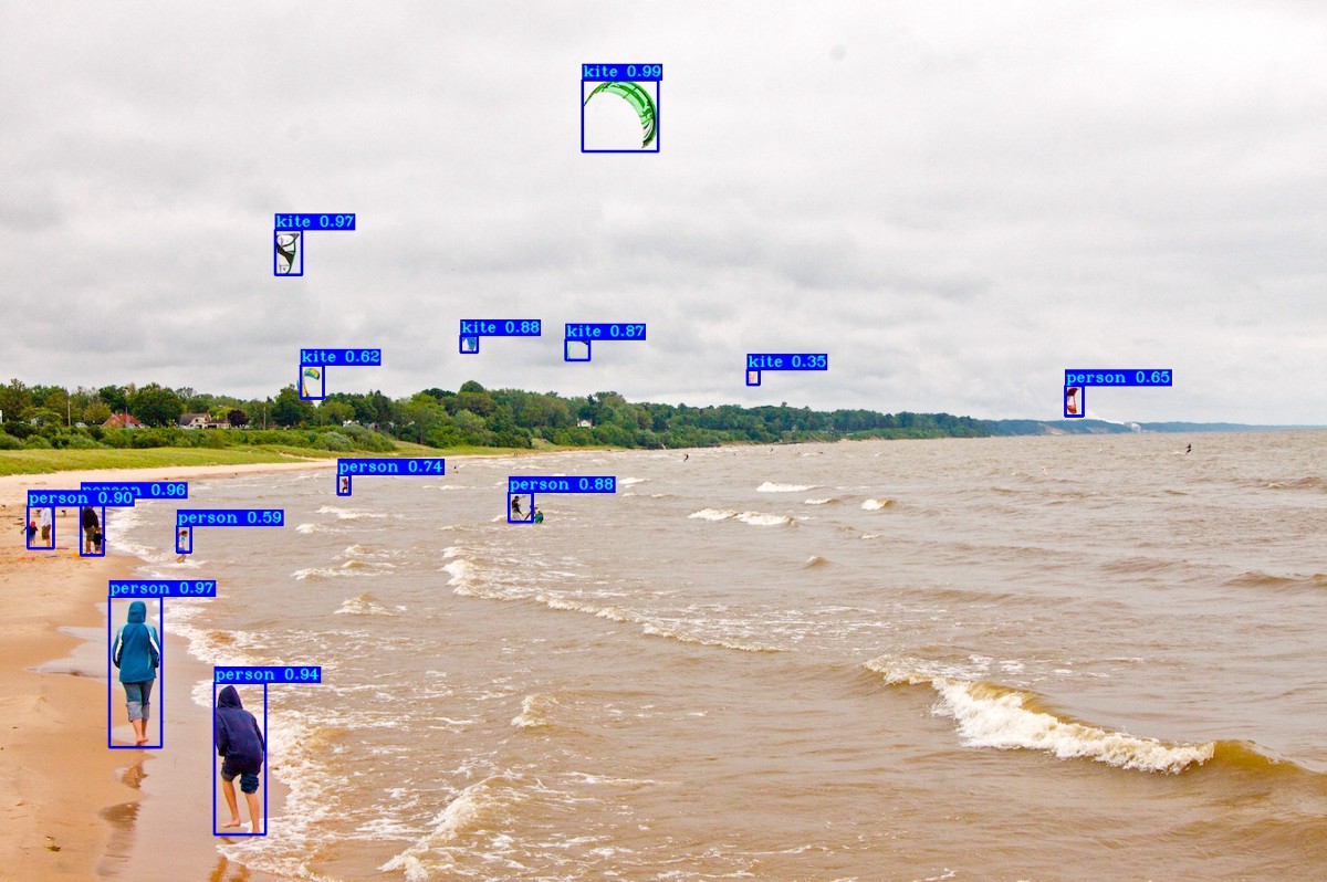 So everything is relatively easy. You can try to use YOLOv4 on video or my object tracking implementation.
YOLOv4 vs. YOLOv3 results
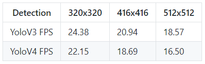
So, one of the most known methods to evaluate and compare model performance is to check the mean average precision on the same data and frames per detection. So, I tried to assess both models with 320, 416, and 512 input images sizes. All tests were done on my 1080TI GPU, with zero overclocking and 300W power, so here are the results for detection speed:
Here are the results for the mAP (mean average precision):
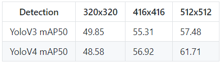 So, these are my results, to make a more accurate generalization, we would need to do more testings, but it's enough to make your own initial opinion about YOLOv4. We can see that YOLOv4 performance significantly increase when we use an input image with 512x512 size. Maybe I have something wrong implemented in my evaluation function, I can't tell you, but if someone finds any mistakes and reports them on GitHub, I will fix it! So, don't hesitate to do that. Moreover, I will be working on this project for quite some time to fix all issues.
Conclusion:
So, if you've made it this far and reading this conclusion - congrats! But this is not the end; this is the only first part. The next part will be about training. If you are trying to understand a YOLOv4 paper, it's tough to understand everything only from it. To get a deep understanding, you need to read many papers, blogs, and code implementations.
While this post mainly presents what technologies have been integrated into YOLOv4, after reading it, you should understand that YOLOv4 authors have spent a lot of effort in evaluating other technologies to make it work.
So, I hope this tutorial will be helpful to you, and if you liked it you like it, share it and see you in the next Bag-Of-Specials part!