The YOLO object detector is often cited as one of the fastest deep learning-based object detectors, achieving a higher FPS rate than computationally expensive two-stage detectors (ex. Faster R-CNN) and some single-stage detectors (ex. RetinaNet and some, but not all, variations of SSDs).
However, even with all that speed, YOLOv3 is still not fast enough to run on some specific tasks or embedded devices such as the Raspberry Pi.
To help make YOLOv3 even faster, Redmon et al. (the creators of YOLO), defined a variation of the YOLO architecture called YOLOv3-Tiny.
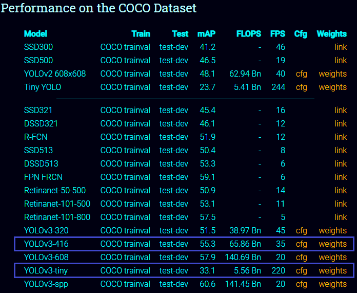
Looking at the results from pjreddie.com (image below), the YOLOv3-Tiny architecture is approximately six times faster than its larger big brothers, achieving upwards of 220 FPS on a single GPU.
The small model size and fast inference speed make the YOLOv3-Tiny object detector naturally suited for embedded computer vision/deep learning devices such as the Raspberry Pi, Google Coral, NVIDIA Jetson Nano, or desktop CPU computer where your task requires a higher FPS rate than you can get with original YOLOv3 model.
In this post, you'll learn how to use and train YOLOv3-Tiny the same way we used it in my previous tutorials.
The downside, of course, is that YOLOv3-Tiny tends to be less accurate because it is a smaller version of its big brother.
For reference, Redmon et al. report ~51–58% mAP for YOLOv3 on the COCO benchmark dataset while YOLOv3-Tiny is only 33.1% mAP — almost less than half of the accuracy of its bigger brothers.
That said, 33% mAP is still reasonable enough for some applications.
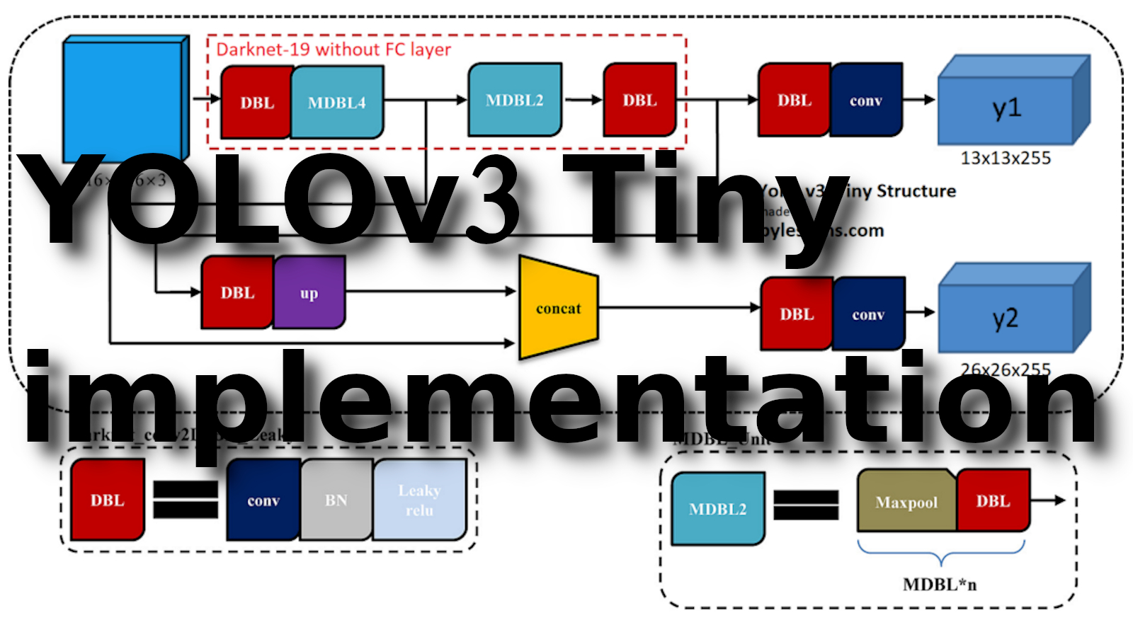
As I said, on a standard computer with a Graphics Processing Unit (GPU), it is easy for YOLOv3 to achieve real‐time performance. However, in the miniaturized embedded devices, such as Raspberry PI, the conventional YOLOv3 algorithm runs slowly. The YOLOv3‐Tiny network can satisfy real‐time requirements based on limited hardware resources. Therefore, in this tutorial, I will show you how to run the YOLOv3‐Tiny algorithm. YOLOv3‐Tiny instead of Darknet53 has a backbone of the Darknet19. The structure of it is shown in the following image:
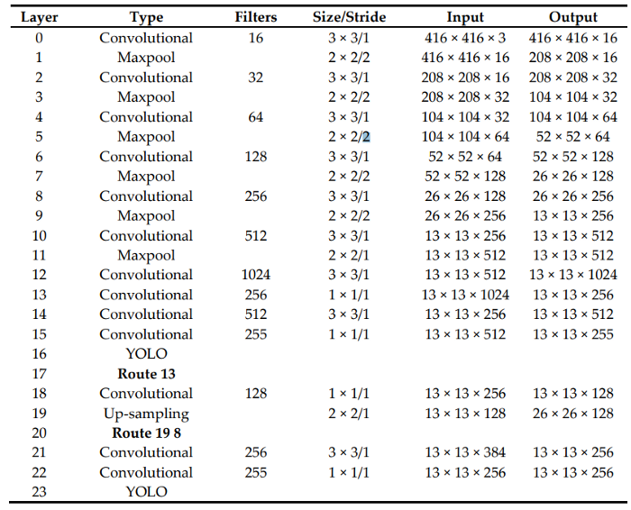
The above structure enables the YOLOv3‐Tiny network to achieve the desired effect in miniaturized devices.
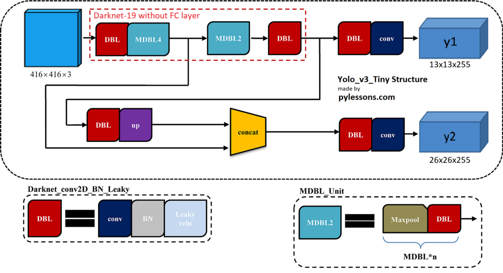
Same as in the YOLOv3 tutorial, seeing Darknet-19 and above YOLOv3-Tiny structure, we can't fully understand all layers and how to implement it. This is why I have one more figure with the overall architecture of the YOLOv3-Tiny network. The picture below shows that the input picture of size 416x416 gets two branches after entering the Darknet-19 network. These branches undergo a series of convolutions, upsampling, merging, and other operations. Two feature maps with different sizes are finally obtained, with shapes of [13, 13, 255] and [26, 26, 255]:
To see the full YOLOv3-Tiny implementation, you can check my GitHub repository. The whole model was divided into three darknet19_tiny, YOLOv3_tiny, and Create_Yolov3 functions:
def darknet19_tiny(input_data):
    input_data = convolutional(input_data, (3, 3, 3, 16))
    input_data = MaxPool2D(2, 2, 'same')(input_data)
    input_data = convolutional(input_data, (3, 3, 16, 32))
    input_data = MaxPool2D(2, 2, 'same')(input_data)
    input_data = convolutional(input_data, (3, 3, 32, 64))
    input_data = MaxPool2D(2, 2, 'same')(input_data)
    input_data = convolutional(input_data, (3, 3, 64, 128))
    input_data = MaxPool2D(2, 2, 'same')(input_data)
    input_data = convolutional(input_data, (3, 3, 128, 256))
    route_1 = input_data
    input_data = MaxPool2D(2, 2, 'same')(input_data)
    input_data = convolutional(input_data, (3, 3, 256, 512))
    input_data = MaxPool2D(2, 1, 'same')(input_data)
    input_data = convolutional(input_data, (3, 3, 512, 1024))

    return route_1, input_data

def YOLOv3_tiny(input_layer, NUM_CLASS):
    # After the input layer enters the Darknet-53 network, we get three branches
    route_1, conv = darknet19_tiny(input_layer)

    conv = convolutional(conv, (1, 1, 1024, 256))
    conv_lobj_branch = convolutional(conv, (3, 3, 256, 512))

    # conv_lbbox is used to predict large-sized objects , Shape = [None, 26, 26, 255]
    conv_lbbox = convolutional(conv_lobj_branch, (1, 1, 512, 3*(NUM_CLASS + 5)), activate=False, bn=False)

    conv = convolutional(conv, (1, 1, 256, 128))
    # upsample here uses the nearest neighbor interpolation method, which has the advantage that the
    # upsampling process does not need to learn, thereby reducing the network parameter
    conv = upsample(conv)

    conv = tf.concat([conv, route_1], axis=-1)
    conv_mobj_branch = convolutional(conv, (3, 3, 128, 256))
    # conv_mbbox is used to predict medium size objects, shape = [None, 13, 13, 255]
    conv_mbbox = convolutional(conv_mobj_branch, (1, 1, 256, 3 * (NUM_CLASS + 5)), activate=False, bn=False)

    return [conv_mbbox, conv_lbbox]

def Create_Yolov3(input_size=416, channels=3, training=False, CLASSES=YOLO_COCO_CLASSES):
    NUM_CLASS = len(read_class_names(CLASSES))
    input_layer  = Input([input_size, input_size, channels])

    if TRAIN_YOLO_TINY:
        conv_tensors = YOLOv3_tiny(input_layer, NUM_CLASS)
    else:
        conv_tensors = YOLOv3(input_layer, NUM_CLASS)

    output_tensors = []
    for i, conv_tensor in enumerate(conv_tensors):
        pred_tensor = decode(conv_tensor, NUM_CLASS, i)
        if training: output_tensors.append(conv_tensor)
        output_tensors.append(pred_tensor)

    YoloV3 = tf.keras.Model(input_layer, output_tensors)
    return YoloV3
If you are interested in how other code parts work, you should check my first tutorial, where I explain YOLOv3 theory because it's quite the same.
Test YOLOv3-Tiny detection:
So, you may ask how to switch from YOLOv3 to YOLOv3-Tiny. In the yolov3 folder, the answer is simple: open configs.py scripts and change TRAIN_YOLO_TINY from False to True. Of course, you may change other parameters the same way as I did in my previous tutorials for YOLOv3.
To test if detection works for you, run the detection_demo.py script. The default image path is kite.jpg, so you should see detections on this image:
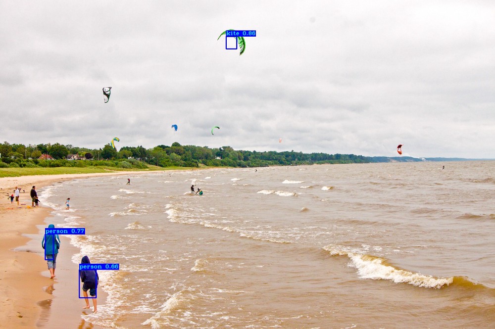 If we compared results with the original YOLOv3 model, I would say that it performs much worse. In my YouTube tutorial, I ran this tiny model on video. It receives around 34 FPS on Nvidia 1080TI, that's around 70% faster than big brother. But detection accuracy is much worse, so before using it, you should decide that you need speed (YOLOv3-Tiny) or accuracy (YOLOv3).
Train custom YOLOv3-Tiny model:
Now, as well as we did for the YOLOv3 model, the best way to test if custom model training works, train it on my already prepared Mnist dataset. If you want to train it on a custom dataset, you can check my previous tutorial.
When you have cloned the GitHub repository, you should see the "mnist" folder containing mnist images. From their images, we create mnist training data with the following command: python mnist/make_data.py.
This make_data.py script creates training and testing images in a suitable format. Also, this makes an annotation file.
The yolov3/configs.py file is already configured for mnist training, but you need to change these settings to train the Tiny model.
Now, you can train and evaluate your YOLOv3-Tiny model:
python train.py
tensorboard --logdir=log
After my model finished the training, in Tensorboard I saw the following results:
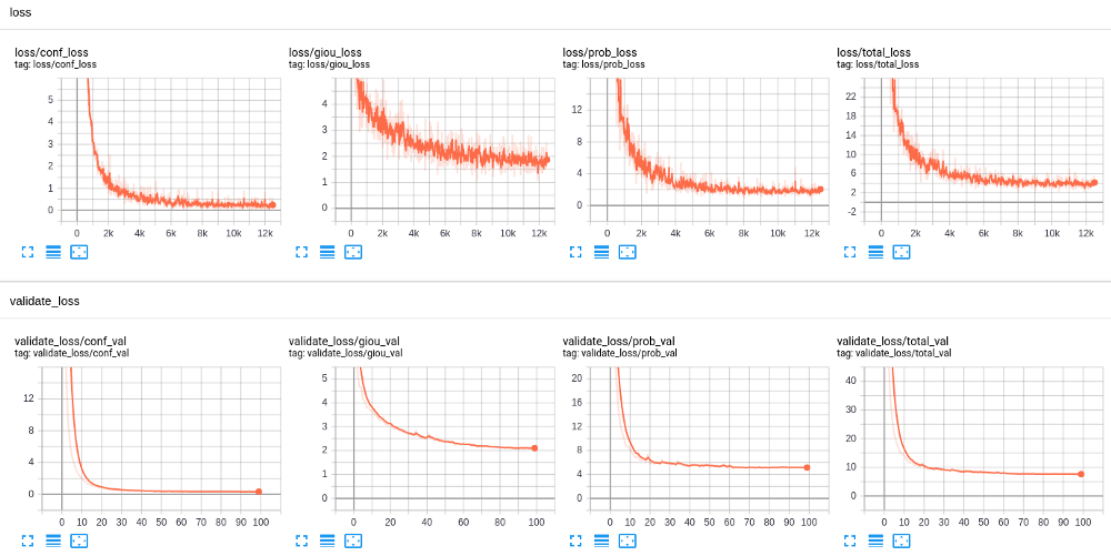
These were quite lovely results, but only because mnist is quite a simple dataset. As well, while training the YOLOv3 model, I used to train for 30 epochs. A tiny model was required to train it for 100 epochs. This means that we need to train a tiny model for more epochs than the original one.
Our new custom model is saved in the checkpoints folder as yolov3_custom_tiny. To check how detection works on our mnist custom detector, run detect_mnist.py script with yolov3_custom_tiny weights. I ran this script and received the following results:
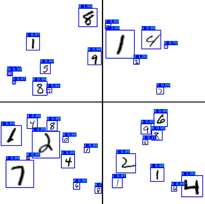
From the results, we can see that for mnist custom, Tiny detection works quite accurately, but this may be only because it's quite a simple dataset. If you would like to train and run a detector for the custom YOLOv3-Tiny model on different datasets, check my previous tutorial to show how to prepare it for training.
Conclusion:
I haven't tested to train a tiny custom model on different custom datasets than mnist, but if it worked on mnist, I don't see why it shouldn't work on a different dataset. In code, I made a workaround (ANCHORS AND STRIDES) to use the YOLOv3-Tiny model because it's used much fewer times than the original one, and I didn't want to invest a lot of time to do massive code changes because this requires a lot of time. Maybe in the future, I will make changes that we won't need a workaround. Now you can test this code on low-end devices. If you find any mistakes in code or you have a suggestion on how to improve it, don't hesitate to make a pull request on GitHub!
If you need more accuracy from the Tiny model, on Google, you can find many articles with modified versions and what strategies people use to make it better. But this wasn't the goal of this tutorial.
Thanks for reading, and see you in the next part.