BipedalWalker-v3 with Continuous Proximal Policy Optimization

In this tutorial, we'll learn more about continuous Reinforcement Learning agents and how to teach BipedalWalker-v3 to walk! First of all, I should mention that this tutorial continues my previous tutorial, where I covered PPO with discrete actions.

To develop a continuous action space Proximal Policy Optimization algorithm, we must first understand their difference. Because LunarLander-v2 environment also has a continuous environment called LunarLanderContinuous-v2, I'll mention what the difference between them is:

• LunarLander-v2 has a Discrete(4) action space. This means there are four outputs (left engine, right engine, main engine, and do nothing), and we send to the environment which one we want to execute. So in practice, we pick the action with the biggest value and send to the environment one number from 0 to 3;
• LunarLanderContinuous-v2 has a Box(2) output. This means there are two continuous outputs, where we need to send both outputs, which will control the ship. The first one controls the main engine, and the second one controls the left and right engines. The expected range of the output is Box[-1..1, -1..1], so we need to normalize the network to give us values inside that range (using TanH, for example).

Here is the quote from the LunarLanderContinuous-v2 gym website:

Landing pad is always at coordinates (0,0). Coordinates are the first two numbers in state vector. Reward for moving from the top of the screen to landing pad and zero speed is about 100..140 points. If lander moves away from landing pad it loses reward back. Episode finishes if the lander crashes or comes to rest, receiving additional -100 or +100 points. Each leg ground contact is +10. Firing main engine is -0.3 points each frame. Solved is 200 points. Landing outside landing pad is possible. Fuel is infinite, so an agent can learn to fly and then land on its first attempt. Action is two real values vector from -1 to +1. First controls main engine, -1..0 off, 0..+1 throttle from 50% to 100% power. Engine can't work with less than 50% power. Second value -1.0..-0.5 fire left engine, +0.5..+1.0 fire right engine, -0.5..0.5 off. 

But this tutorial is not about LunarLanderContinuous-v2; now we'll try to learn to control two legs BipedalWalker robot!

Introduction

Reinforcement Learning in the real world is still an ill-defined problem. The agent has to be greedy, but not too greedy... One might conjecture that an optimal agent should have bayesian behavior, which again is not always what we want, nor the design goal of our brain. We want the agent to be curious to exploit the environment whenever possible but not too curious to continue to work for us.

If you were the head of a company, it could all be compared to training your employee. You want your employee to be exceptionally efficient at his job, while at the same time you want them to stay working for you. Which is hard, if not impossible. (unless you're Google… of course)

BipedalWalker-v3 environment

BipedalWalker-v3 is a challenging environment in the Gym. Your agent should run very fast, should not trip himself off, should use as little energy as possible. If you were checking the link, you might have noticed that it's v2, not v3, that I wrote. But this is because Gym didn't update the link; installing the v2 environment doesn't work…

It's pretty hard to find online, what does it mean "Solving" environment, but I found it! The environment requires an average total reward of over 300 over 100 consecutive episodes to be considered as finished, which is incredibly difficult (less than ten people solved it on Gym). I am unsure if the results are legit and official, but I found them on the following GitHub page.

My implemented PPO agent on this tutorial can't break the 300 score mark, but I hope to do that next. Simply while training my agent, the performance stops improving, and from time to time, the agent starts making stupid mistakes and falls; this repeats repeatedly.

Environment and walking strategies

Here is the quote from the openAI wiki page:

Reward is given for moving forward, total 300+ points up to the far end. If the robot falls, it gets -100. Applying motor torque costs a small amount of points, more optimal agent will get better score. State consists of hull angle speed, angular velocity, horizontal speed, vertical speed, position of joints and joints angular speed, legs contact with ground, and 10 lidar rangefinder measurements. There's no coordinates in the state vector. 

Observation

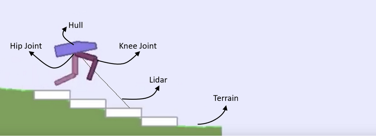
Usually, when programming a standard Reinforcement Learning agent, we don't care what the observation space is. Our agent should fit to whatever it is, but it's better to know the inputs if our agent is not learning. So here is the observation table from the same link I mentioned above, with 24 different parameters in one state:

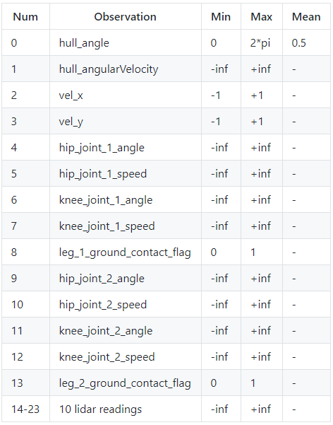
Also, if you paid attention to the above environment image and observation space table, you may have noticed that there is no information about the terrain in the state. This means that our agent doesn't know anything about the way where he is running. He must use lidar to scan the landscape (I think so).

Action Space

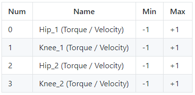
BipedalWalker has two legs. Each leg has two joints. You have to teach the Bipedal-walker to walk by applying the torque on these joints. Therefore the size of our action space is four which is the torque applied on four joints. You can use the torque in the range of (-1, 1), as shown in the following table:

Reward

• The agent gets a positive reward proportional to the distance walked on the terrain. It can get a total of 300+ reward points up to the end;
• If the agent tumbles, it gets a negative reward of -100;
• There is some negative reward proportional to the torque applied on the joint. So that agent learns to walk smoothly with minimal torque.

Also, I must mention that there are two versions of the Bipedal environment based on terrain type:

• Slightly uneven terrain (BipedalWalker-v3);
• Hardcore terrain with ladders, stumps, and pitfalls (BipedalWalkerHardcore-v3).

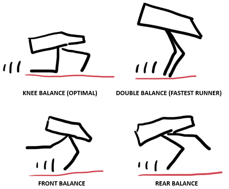
Walking strategies

There are four primary strategies to walk. Usually, our agent tries all of them during the training process:

Same as in my previous tutorial, before moving ahead, let's implement this for a random-action AI agent interacting with this environment. Create a new python file named BipedalWalker-v2_random.py by copying and executing the following code:

import gym
import random
import numpy as np

env = gym.make("BipedalWalker-v3")

def Random_games():
    # Each of this episode is its own game.
    action_size = env.action_space.shape[0]
    for episode in range(10):
        env.reset()
        # this is each frame, up to 500...but we wont make it that far with random.
        while True:
            # This will display the environment
            # Only display if you really want to see it.
            # Takes much longer to display it.
            env.render()
            
            # This will just create a sample action in any environment.
            # In this environment, the action can be any of one how in list on 4, for example [0 1 0 0]
            action = np.random.uniform(-1.0, 1.0, size=action_size)

            # this executes the environment with an action, 
            # and returns the observation of the environment, 
            # the reward, if the env is over, and other info.
            next_state, reward, done, info = env.step(action)
            
            # lets print everything in one line:
            #print(reward, action)
            if done:
                break
                
Random_games()

In the above code, the main code line is: action = np.random.uniform(-1.0, 1.0, size=action_size), where four random numbers between -1 and 1 are generated in NumPy list form:

[ 0.79471074 -0.06168061 0.55740988 -0.74866494]
[ 0.98315975 0.73440604 -0.99219407 -0.966013 ]
[ 0.96877238 0.83464859 -0.47381784 -0.79399857]
[-0.84639089 -0.97504654 0.75642557 -0.95554083]
[ 0.4511413 -0.26661095 -0.36721001 0.20417917]
[ 0.15117511 0.32102874 0.14429348 -0.96409202]
[-0.31694119 -0.9644246 -0.89420344 0.92559095]

Now you should understand why this environment is called continuous, and there might be thousands of values between -1 and 1 where the Actor should decide what action is best. These numbers control our robot legs, it doesn't make a lot of sense for us, but for our AI agent, it will do! We successfully ran BipedalWalker random environment, and now we can implement our PPO algorithm for continuous action space.

The Continuous Actor-Critic model's structure

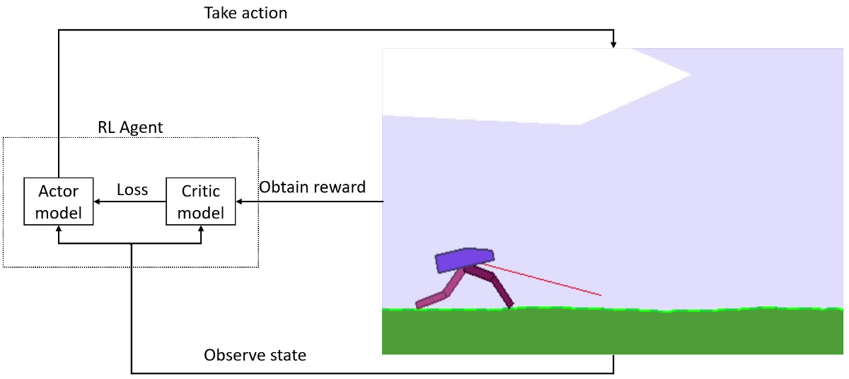
The same as discrete PPO environments, continuous also uses the Actor-Critic approach for the agent. This means that it uses two models, one called the Actor and the other called Critic:

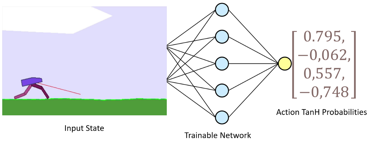
The Actor model

The Actor model performs the task of learning what action to take under a particular observed state of the environment. In the BipedalWalker-v3 case, it takes 24 values list (mentioned before) of the game as input which represents the current state of our walker and gives particular actions what legs to move:

Let's implement this by creating an Actor class:

class Actor_Model:
    def __init__(self, input_shape, action_space, lr, optimizer):
        X_input = Input(input_shape)
        self.action_space = action_space
        
        X = Dense(512, activation="relu", kernel_initializer=tf.random_normal_initializer(stddev=0.01))(X_input)
        X = Dense(256, activation="relu", kernel_initializer=tf.random_normal_initializer(stddev=0.01))(X)
        X = Dense(64, activation="relu", kernel_initializer=tf.random_normal_initializer(stddev=0.01))(X)
        output = Dense(self.action_space, activation="tanh")(X)

        self.Actor = Model(inputs = X_input, outputs = output)
        self.Actor.compile(loss=self.ppo_loss_continuous, optimizer=optimizer(lr=lr))
        #print(self.Actor.summary())

    def ppo_loss_continuous(self, y_true, y_pred):
        advantages, actions, logp_old_ph, = y_true[:, :1], y_true[:, 1:1+self.action_space], y_true[:, 1+self.action_space]
        LOSS_CLIPPING = 0.2
        logp = self.gaussian_likelihood(actions, y_pred)

        ratio = K.exp(logp - logp_old_ph)

        p1 = ratio * advantages
        p2 = tf.where(advantages > 0, (1.0 + LOSS_CLIPPING)*advantages, (1.0 - LOSS_CLIPPING)*advantages) # minimum advantage

        actor_loss = -K.mean(K.minimum(p1, p2))

        return actor_loss

    def gaussian_likelihood(self, actions, pred): # for keras custom loss
        log_std = -0.5 * np.ones(self.action_space, dtype=np.float32)
        pre_sum = -0.5 * (((actions-pred)/(K.exp(log_std)+1e-8))**2 + 2*log_std + K.log(2*np.pi))
        return K.sum(pre_sum, axis=1)

    def predict(self, state):
        return self.Actor.predict(state)

If we were comparing our current Actor and its custom continuous loss function with the discrete PPO actor model, we would see two main differences:

• In a discrete PPO network, our model has "softmax" activation within output in the last layer: output = Dense(self.action_space, activation="softmax")(X)
• In a continuous PPO network, we use TanH instead: output = Dense(self.action_space, activation="tanh")(X). Also, we can remove the activation function at all, but then we don't know what output our model will give to us; it might give us actions outside of our action space limits.
• And the main difference is the custom PPO loss function, which is hard to explain and understand… But I will try.

Continuous PPO loss

The action space defines the distribution used for action selection. The distribution is used to sample/select the action based on the specific distribution, and for a given action, the distribution defines its probability which is plugged into the formula:

$L(s, a, {\theta }_k, \theta )=min\left(\frac{{\pi }_Q\left(a_t\right|s_t)}{{\pi }_{Q_k}\left(a_t\right|s_t)}{A}^{{\pi }_{{\theta }_k}}(s, a), clip\left(\frac{{\pi }_Q\left(a_t\right|s_t)}{{\pi }_{Q_k}\left(a_t\right|s_t)},1-\in ,1+\in \right)A^{{\pi }_{{\theta }_k}}(s, a)\right)$

Above is the PPO probability formula. The distribution usually gives us the 'log prob', and we plug it into the loss using exp(). So it's the same formula in both cases (PPO discrete and continuous); the distribution defines the action selection and its probability.

For discrete action spaces, we have n linear outputs and a categorical distribution. i.e., the outcomes are the logits that define the probabilities using softmax, and we sample based on those. In discrete action space cases, the likelihood is just the softmax value of the chosen action.

Continuous action spaces use normal/gaussian distribution. In this case, the model output is the mean+std which defines the normal distribution for the action selection. The action is sampled from this distribution. In this case, the probability of the action's value under the given normal distribution. I don't understand all the math behind this, or I am not sure if I understand, so I decided not to try explaining it and mislead you into a lousy direction while understanding it. Also, I borrowed the idea of how to implement the Gaussian likelihood function into my code from the stable-baselines GitHub page. But, I couldn't understand how to implement the log_std parameter into my TF2 code, so I used a simpler version of it as a constant parameter. If you have an idea of how to implement log_std I am open to your suggestions. Maybe in the future, I'll find a better way how to do that. I am sure that this parameter is responsible for continuous action space randomness; I'll show this to you later.

The Critic model

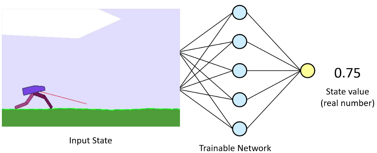
The primary role of the Critic in continuous action space doesn't change from discrete: model is learning to evaluate if the action taken by the Actor led our environment to be in a better state or not and give its feedback to the Actor.

Same as before, we send the action predicted by the Actor to our environment and observe what happens in the game. If something positive happens due to our action, the environment sends back a positive response in the form of a reward and vice versa if we receive a negative reward. These rewards are taken in by training our Critic model:

Action picking

When we go from discrete action space to continuous, we must change the code part where we choose an action. First, I'll give a code part to make sense what is the difference between them:

def act_continuous(self, state):
    # Use the network to predict the next action to take, using the model
    pred = self.Actor.predict(state)

    low, high = -1.0, 1.0 # -1 and 1 are boundaries of tanh
    action = pred + np.random.uniform(low, high, size=pred.shape) * self.std
    action = np.clip(action, low, high)

    logp_t = self.gaussian_likelihood(action, pred, self.log_std)

    return action, logp_t

def gaussian_likelihood(self, action, pred, log_std):
    # https://github.com/hill-a/stable-baselines/blob/master/stable_baselines/sac/policies.py
    pre_sum = -0.5 * (((action-pred)/(np.exp(log_std)+1e-8))**2 + 2*log_std + np.log(2*np.pi)) 
    return np.sum(pre_sum, axis=1)

def act_discrete(self, state):
    # Use the network to predict the next action to take, using the model
    prediction = self.Actor.predict(state)[0]
    action = np.random.choice(self.action_size, p=prediction)
    action_onehot = np.zeros([self.action_size])
    action_onehot[action] = 1
    return action, action_onehot, prediction

So, here is an example, what happens in discrete action space:

pred = np.array([0.05, 0.85, 0.1]) 
action_size = 3 
action = np.random.choice(a, p=pred) 
action = 1

result: >>> 1, because it has the highest probability to be taken, while in continuous we receive the following:

std = 0.3 # example number
random_uniform = [0.5, -0.7, 0.1, 0.9]
pred = [0.79471074, -0.06168061, 0.55740988, -0.74866494]
action = pred + random_uniform * std
action = [0.94471074, -0.27168061, 0.58740988, -0.47866494]

So, these are examples for better understanding. Also, we do a clipping in continuous action space to make sure our actions are between -1 ar 1 boundaries. For training, we calculate log_pt with the Gaussian Likelihood, as I mentioned before.

Model Training

When we have covered most differences from discrete action space, we can finally start the model training. For this, I use mostly known the fit function of Keras in the following code:

def replay(self, states, actions, rewards, dones, next_states, logp_ts):
    # reshape memory to appropriate shape for training
    states = np.vstack(states)
    next_states = np.vstack(next_states)
    actions = np.vstack(actions)
    logp_ts = np.vstack(logp_ts)

    # Get Critic network predictions 
    values = self.Critic.predict(states)
    next_values = self.Critic.predict(next_states)

    # Compute discounted rewards and advantages
    #discounted_r = self.discount_rewards(rewards)
    #advantages = np.vstack(discounted_r - values)
    advantages, target = self.get_gaes(rewards, dones, np.squeeze(values), np.squeeze(next_values))
    '''
    pylab.plot(adv,'.')
    pylab.plot(target,'-')
    ax=pylab.gca()
    ax.grid(True)
    pylab.subplots_adjust(left=0.05, right=0.98, top=0.96, bottom=0.06)
    pylab.show()
    if str(episode)[-2:] == "00": pylab.savefig(self.env_name+"_"+self.episode+".png")
    '''
    # stack everything to numpy array
    # pack all advantages, predictions and actions to y_true and when they are received
    # in custom loss function we unpack it
    y_true = np.hstack([advantages, actions, logp_ts])

    # training Actor and Critic networks
    a_loss = self.Actor.Actor.fit(states, y_true, epochs=self.epochs, verbose=0, shuffle=self.shuffle)
    c_loss = self.Critic.Critic.fit([states, values], target, epochs=self.epochs, verbose=0, shuffle=self.shuffle)

    # calculate loss parameters (should be done in loss, but couldn't find working way how to do that with disabled eager execution)
    pred = self.Actor.predict(states)
    log_std = -0.5 * np.ones(self.action_size, dtype=np.float32)
    logp = self.gaussian_likelihood(actions, pred, log_std)
    approx_kl = np.mean(logp_ts - logp)
    approx_ent = np.mean(-logp)

    self.writer.add_scalar('Data/actor_loss_per_replay', np.sum(a_loss.history['loss']), self.replay_count)
    self.writer.add_scalar('Data/critic_loss_per_replay', np.sum(c_loss.history['loss']), self.replay_count)
    self.writer.add_scalar('Data/approx_kl_per_replay', approx_kl, self.replay_count)
    self.writer.add_scalar('Data/approx_ent_per_replay', approx_ent, self.replay_count)
    self.replay_count += 1

From the above code, you can see that everything is quite the same, except that instead of collecting predictions as we did in discrete action space, right now, we collect logp_ts. We stack advantages, actions and logp_ts to the NumPy array, and we send these stacked variables to our custom PPO loss function while calling a fit function. After a fit function, you can see a little more code, but this is only for graphs to track our model training performance.

To glue everything to one working and straightforward code took me a few weeks, with many experiments. But right now, I can proudly announce that to train BipedalWalker-v3 is not hat hard task as it looked for me in the first days.

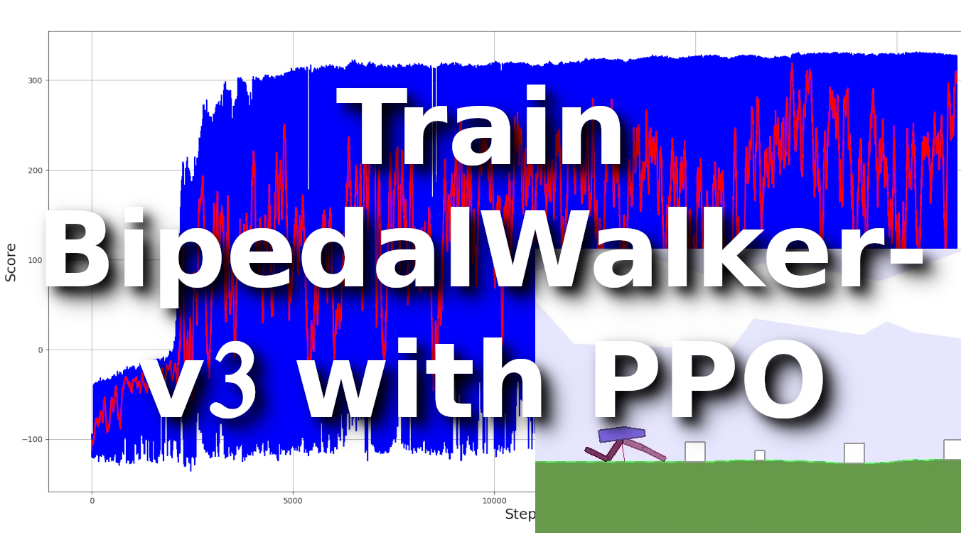
My code took only 6k training steps to achieve maximum results, where 50 episodes moving average score was close to 300, running it on test environment was even better! So, here is the training graph:

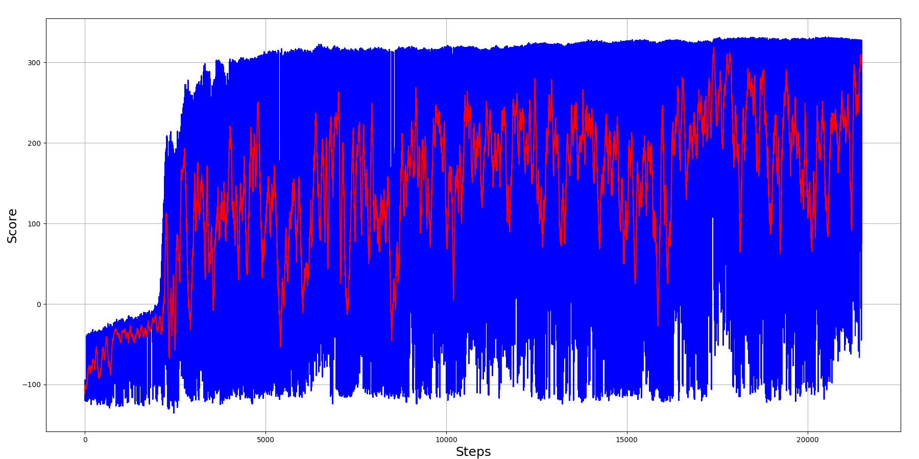
As we can see from the above chart, the most challenging task was to learn that we needed to move forward somehow; this took around 1k training steps. When our agent understood that he needed to move forward as fast as possible, he started learning the above walking strategies. After around 4k training steps, our agent was able to get around a maximum of 300 score. And as we can see, the 50 moving average is near 300, that's a fantastic result!

After training my agents, I decided to check if my agent can complete 100 episodes with an average score above 300:

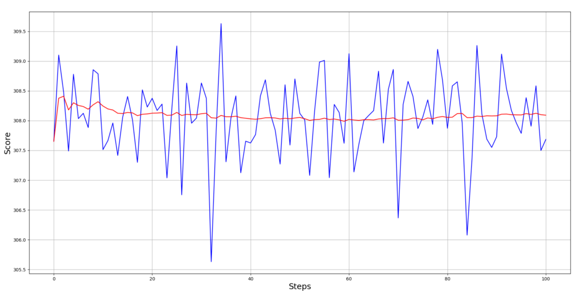
The results show that my moving average is above the 300 scorelines; this is even better than I thought!

Conclusion:

For quite a long time, I could not understand the differences between discrete and continuous action spaces in PPO. This BipedalWalker-3 tutorial motivated me to understand better how everything works and how I can implement everything from scratch. By the way, Gym environments are a great place to test how our algorithm implementations work; without Gym, I think it wouldn't be so easy. This continuous environment still has few areas where I can improve it, but I am proud to give you my working code depending on the results I obtained. I would appreciate your suggestions on how I could implement Gaussian likelihood correctly, but anyway, I will try to do it in my spare time, even without your suggestions.

Anyway, I learned a lot while writing this tutorial, and I think in the future while working on other projects, I am sure I will do them based on this code. There is still a BipedalWalkerHardcore-v3 environment that I could finish, so maybe I will play around with it before moving to the next project.

I hope this tutorial will explain the continuous PPO model and how to implement it. Do not hesitate to clone my GitHub repository and test it by yourself! See you in the next part!