Solving the Cartpole with Dueling Double Deep Q Network

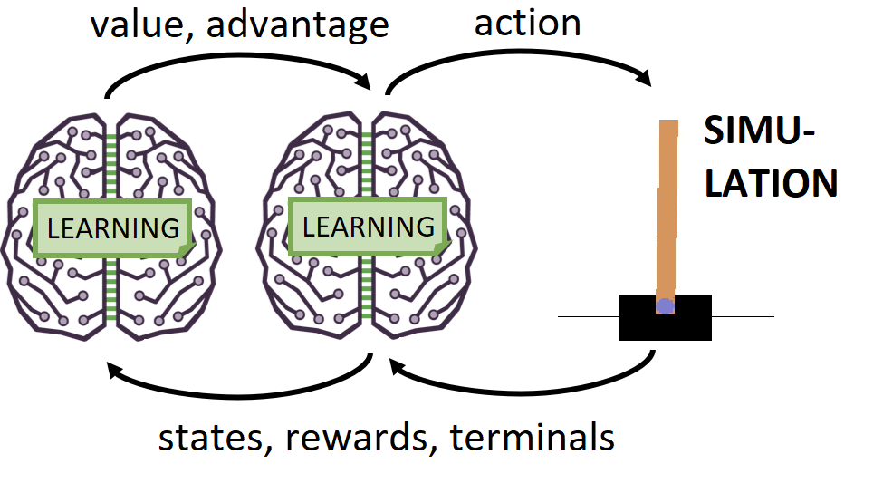
Dueling DQN introduction

In this post, we'll be covering Dueling DQN Networks for reinforcement learning. This reinforcement learning architecture is an improvement from our previous tutorial (Double DQN) architecture, so before reading this tutorial, I recommend you read my previous tutorials. This tutorial will introduce the Dueling Deep Q Network architecture (D3QN), its advantages, and how to build one in Keras. We'll be running the code on the same Open AI gym's CartPole environment so that everyone could train and test the network quickly and easily.

In future tutorials, I'll be testing this code on more complicated games that will need Convolutional Neural Networks. To introduce reinforcement learning, I recommend checking out my previous tutorials. All the code for this and previous tutorials can be found on this site's GitHub repo.

Double DQN introduction

To get a deeper understanding of Dueling Network, we should recap some points from Double Q learning. As discussed in the previous DDQN tutorial, vanilla deep Q learning has some problems. These problems can be separated into two main issues:

• DQN Networks tend to overestimate rewards in noisy environments, leading to non-optimal training outcomes;
• The moving target problem is that the same network is responsible for choosing and evaluating actions, leading to training instability.

Regarding the 1st point – for example, if we have a state with two possible actions, each giving rewards with a noise. The first action returns a random reward based on a normal distribution with a mean of two and a standard deviation of 1 – N(2, 1). The second action returns a random reward from a normal distribution of N(1, 4). As a result, action a is the optimal action to take in this state. Still, because of the argmax function in deep Q learning, action b tends to favor higher standard deviation / higher random rewards.

Regarding the 2nd point – let's imagine another state, with three possible actions a, b, and c. Let's assume we know that b is the optimal action. But when we first initialize the Neural Network, in state 1, action tends to be chosen. When we train Neural Network, the loss function will drive the network's weights to choose action b. However, we are in state 1, and the network parameters have changed so much that action c is chosen. 

This problem arises when we are choosing actions and evaluating them with the same network. In the ideal situation, we would like our Neural Network to consistently choose action in one state until it was gradually trained to choose action b. But now, the goal has shifted, and we want to move the Network goal from c to b instead of a to b – this causes instability in training.

To solve this problem, Double Q learning proposed the following way of determining the target Q value:

${\mathrm{Q}}_{\mathrm{target}}={\mathrm{r}}_{\mathrm{t}\mathit{+}1}\mathit{+}\mathrm{yQ}({\mathrm{s}}_{\mathrm{t}\mathit{+}1}, \mathrm{argmaxQ}({\mathrm{s}}_{\mathrm{t}\mathit{+}1}, \mathrm{a}; {\mathrm{\theta }}_{\mathrm{t}});{\mathrm{\theta }}_{\mathrm{t}}^{-})$

This target network is a copy of the primary network. Here θt refers to the primary network parameters (weights) at time t, and θt with minus refers to the target network parameters at time t. As can be seen, the optimal action in state t+1 is chosen from the primary network θt. Still, the evaluation or estimate of the Q value of this action is determined from the target network θt. This can be illustrated more clearly by the following equations:

$$\begin{gathered} a=argmaxQ(s_{t+1}, a, {\theta }_t) \\ {\mathrm{Q}}_{\mathrm{target}}={\mathrm{r}}_{\mathrm{t}\mathit{+}1}\mathit{+}\mathrm{yQ}({\mathrm{s}}_{\mathrm{t}\mathit{+}1}, a; {\mathrm{\theta }}_{\mathrm{t}}^{-}) \end{gathered}$$

By doing this, these two things occur. First, different networks are used to choose and evaluate the actions. This breaks the moving target problem mentioned earlier. Second, the primary network and the target network have essentially been trained on different samples from the memory bank of states and actions (the target network is "trained" on older samples than the primary network). Because of this, any bias due to environmental randomness should be "smoothed out". As was shown in my previous tutorial on Double Q learning, there is a significant improvement in using Double Q learning instead of vanilla deep Q learning. However, a further improvement can be made on the Double Q idea – the Dueling Q architecture, which will be covered next.

Dueling DQN theory

The Dueling DQN architecture trades on the idea that the evaluation of the Q function implicitly calculates two quantities:

• V(s) – the value of being in state s;
• A(s, a) – the advantage of taking action in state s.

Together with the Q function Q(s, a), these values are fundamental to understanding to do a deep dive into these concepts. Let's first examine the generalized formula for the value function V(s):

$V^{\mathrm{\pi }}\left(s\right)=\mathbb{E}\left[\sum _{i=1}^T{y}^{i-1}{r}_i\right]$

The above formula means that the value function at state s, operating under a policy, is the summation of future discounted rewards starting from state s. In other words, if an agent starts at s, it is the sum of all the rewards the agent collects operating under a given policy π. The E is the expectation operator. For example, let's assume an agent is playing a game with a set number of rounds. In the second-to-last round, the agent is in state s. It has three possible actions from this state, with possible 10, 50, and 100 rewards. Let's imagine that the policy for this agent is a simple random selection (this means we pick actions randomly). Because this is the last round of actions and rewards in the game, there are no discounted future rewards due to the game finishing the round. So, the value for this state and the random action policy would be:

$V^{\mathrm{\pi }}\left(s\right)=\mathbb{E}\left[random(10, 50, 100)\right]=53.333$

This policy is not going to produce optimum outcomes. However, we know that for the optimum policy, the best value of this state would be:

V*(s)=max(10, 50, 100)=100

If we recall, from Q learning theory, the optimal action in this state is:

$a=argmaxQ(s_{t+1}, a)$

and the optimal Q value from chosen action in this state would be:

Q(s, a) = max(10, 50, 100) = 100

So, under the optimal (deterministic) policy, we have:

Q(s, a) = V(s)

But what if we aren't operating under the optimal policy (yet)? Let's get back to the case where our policy is simple random action selection. In such a case, the Q function at state s could be described as (remember there is no future discounted rewards, and have:

Q(s, a) = V(s)+(−43.33, −3.33, 46.67) = (10, 50, 100)

Under such an analysis, the term (-43.33, -3.33, 46.67) is called the Advantage function A(s, a). The Advantage function expresses the relative benefits of the various actions possible in state s. The Q function can therefore be expressed as:

Q(s, a) = V(s)+A(s, a)

Under the optimum policy, we have A(s, a) = 0 and V(s) = 100 and the whole result is:

Q(s,a)=V(s)+A(s,a)=100+(−90,−50,0)=(10,50,100)

But why do we want to decompose the Q function in this way? Because there is a difference between the value of a particular state s and the actions proceeding from that state. Consider a game where, from a given state s*, all actions lead to the agent dying and ending the game. This is the state where we want to spend the least time, and who cares what action we'll take in such a state? It is pointless for the learning algorithm to waste time and training resources finding the best actions to take. In such a state, the Q values should be based solely on the value function V, and this state should be avoided. The converse case also holds – some states are just inherently valuable to be in, regardless of the effects of subsequent actions.

Consider below images taken from the original Dueling DQN paper – showing the value and advantage components of the Q value in the Atari game:

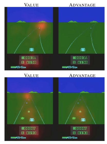
In the Atari Enduro game, the agent's goal is to pass as many cars as possible. Crashing into a car slows the agent's car down and therefore reduces the number of vehicles that will be overtaken. In the images above, it can be observed that the value stream considers the road ahead and the score. However, the advantage stream does not "pay attention" to anything when no cars are visible. It only begins to register when there are cars close by and action is required to avoid them. This is a good outcome, as when no cars are in view, the network should not be trying to determine which actions to take as this is a waste of training resources. This is an excellent example of showing the benefit of splitting value and advantage functions.

If the ML engineer already knows it is essential to separate value and advantage values, why not build them into the network architecture and save the learning algorithm the hassle? That is essentially what the Dueling Q network architecture does. Consider the image below showing the original Dueling DQN architecture:

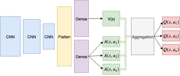
First, notice that the first part of architecture is standard, with CNN input filters and a common Flatten layer (for more on convolutional neural networks, see this tutorial); we will use this architecture later when we'll do something more serious than CardPole. After the flatten layer, the network divides into two separate densely connected layers. The first densely connected layer produces a single output corresponding to V(s). The second densely connected layer has n outputs, where n is the number of available actions – and each of these outputs is the expression of the advantage function. These value and advantage functions are then aggregated in the Aggregation layer to produce Q values estimations for each possible action in state s. These Q values can then be trained to approach the target Q values, generated via the Double Q mechanism, i.e.:

${\mathrm{Q}}_{\mathrm{target}}={\mathrm{r}}_{\mathrm{t}\mathit{+}1}\mathit{+}\mathrm{yQ}({\mathrm{s}}_{\mathrm{t}\mathit{+}1}, \mathrm{argmaxQ}({\mathrm{s}}_{\mathrm{t}\mathit{+}1}, \mathrm{a}; {\mathrm{\theta }}_{\mathrm{t}});{\mathrm{\theta }}_{\mathrm{t}}^{-})$

What goes on in the aggregation layer? One might think we could add the V(s) and A(s, a) values together like so: Q(s, a)=V(s)+A(s, a). The network will learn to produce accurate estimates of the values and advantages through these different value and advantage streams, improving learning performance. However, there is an issue here, and it's called the problem of identifiability. This problem in the current context can be stated as follows: given Q, there is no way to identify V or A uniquely. What does this mean? Say that the network is trying to learn some optimal Q value for action a. Can we uniquely learn a V(s) and A(s, a) value given this Q value? Under the formulation above, the answer is no.

Let's say the "true" value of being in state s is 50, i.e., V(s) = 50. Let's also say the "true" advantage in state s for action a is 10. This will give a Q value, Q(s, a) of 60 for this state and action. However, we can also arrive at the same Q value for a learned V(s) of, say, 0, and an advantage function A(s, a) = 60. Alternatively, a learned V(s) of -1000 and an advantage A(s, a) of 1060. In other words, there is no way to guarantee the "true" values of V(s) and A(s, a) are being learned separately and uniquely from each other. The commonly used solution to this problem is to perform the following aggregation function instead:

$Q(s, a)=V\left(s\right)+A(s, a)-\frac{1}{||a||}\sum _{a\text{'}}A(s, a\text{'})$

Here the advantage function value is normalized concerning the mean of the advantage function values over all actions in state s.

So, we usually create a common network consisting of introductory layers that act to process state inputs. Then, two separate streams are created using densely connected layers, which learn the value and advantage estimates, respectively. These are then combined in a particular aggregation layer that calculates the above equation to arrive at Q values finally. Once the above description specifies the network architecture, the training proceeds in the same fashion as Double Q learning. The agent actions can be selected either directly from the output of the advantage function or the output Q values. Because the Q values differ from the advantage values only by the addition of the V(s) value (which is independent of the actions), the argmax-based selection of the best move will be the same regardless of whether it is extracted from the advantage or the Q values of the network.

Dueling DQN network model

In this part, we will build a Dueling DQN architecture. While Dueling DQN was originally designed for processing images, with its multiple Convolutional layers, in this example, we'll use simple Dense layers instead of using CNN layers. However, we'll write the code in a way that both Double DQN and Dueling DQN networks could be constructed with the simple change of a boolean identifier to compare results easily. Train reinforcement learning agents with CNN layers takes a long time; that's why I decide to simplify architecture for educational purposes. In future tutorials, we will learn how to train the RL model on games like Atari.

So, let's begin with creating a Keras model where we could easily switch between dueling or not dueling DQN model:

def OurModel(input_shape, action_space, dueling):
    X_input = Input(input_shape)
    X = X_input

    # 'Dense' is the basic form of a neural network layer
    # Input Layer of state size(4) and Hidden Layer with 512 nodes
    X = Dense(512, input_shape=input_shape, activation="relu", kernel_initializer='he_uniform')(X)

    # Hidden layer with 256 nodes
    X = Dense(256, activation="relu", kernel_initializer='he_uniform')(X)
    
    # Hidden layer with 64 nodes
    X = Dense(64, activation="relu", kernel_initializer='he_uniform')(X)

    if dueling:
        state_value = Dense(1, kernel_initializer='he_uniform')(X)
        state_value = Lambda(lambda s: K.expand_dims(s[:, 0], -1), output_shape=(action_space,))(state_value)

        action_advantage = Dense(action_space, kernel_initializer='he_uniform')(X)
        action_advantage = Lambda(lambda a: a[:, :] - K.mean(a[:, :], keepdims=True), output_shape=(action_space,))(action_advantage)

        X = Add()([state_value, action_advantage])
    else:
        # Output Layer with # of actions: 2 nodes (left, right)
        X = Dense(action_space, activation="linear", kernel_initializer='he_uniform')(X)

    model = Model(inputs = X_input, outputs = X, name='CartPole Dueling DDQN model')
    model.compile(loss="mean_squared_error", optimizer=RMSprop(lr=0.00025, rho=0.95, epsilon=0.01), metrics=["accuracy"])

    model.summary()
    return model

Let's walk line by line through the above code. First, several parameters are passed to this model as part of its initialization – data input shape, the number of actions in the environment, and finally, a Boolean variable - dueling, to specify whether the network should be a Q network or a Dueling Q network. The first three model layers defined are simple Keras densely connected layers. These layers follow with the ReLU activations and use the He uniform weight initialization technique. If the network is to be a Q network (i.e., dueling == False), then there will be a fourth densely connected layer followed by the output of the third Q layer.

However, if the network is specified to be a Dueling Q network (i.e., dueling == True), then the value and advantage streams are created. Then a final, single dense layer is designed to output the single state_value estimation V(s) for the given state. However, keeping with the Dueling DQN terminology, the last dense layer associated with the action_advantage stream is another standard Dense layer of size = action_space. Each of these outputs will learn to estimate the advantage of all the actions in the given state A(s, a).

$A(s, a)-\frac{1}{||a||}\sum _{a\text{'}}A(s, a\text{'})$

This can be easily calculated by using the lambda function lambda a: a[:, :] - k.mean(a[:, :], keepdims=True) expression in the Lambda layer. Finally, we use a simple Keras addition layer to add this mean-normalized advantage function to the value estimation. This completes the explanation of our defined model function.

Full tutorial code from GitHub:

# Tutorial by www.pylessons.com
# Tutorial written for - Tensorflow 1.15, Keras 2.2.4

import os
import random
import gym
import pylab
import numpy as np
from collections import deque
from keras.models import Model, load_model
from keras.layers import Input, Dense, Lambda, Add
from keras.optimizers import Adam, RMSprop
from keras import backend as K

def OurModel(input_shape, action_space, dueling):
    X_input = Input(input_shape)
    X = X_input

    # 'Dense' is the basic form of a neural network layer
    # Input Layer of state size(4) and Hidden Layer with 512 nodes
    X = Dense(512, input_shape=input_shape, activation="relu", kernel_initializer='he_uniform')(X)

    # Hidden layer with 256 nodes
    X = Dense(256, activation="relu", kernel_initializer='he_uniform')(X)
    
    # Hidden layer with 64 nodes
    X = Dense(64, activation="relu", kernel_initializer='he_uniform')(X)

    if dueling:
        state_value = Dense(1, kernel_initializer='he_uniform')(X)
        state_value = Lambda(lambda s: K.expand_dims(s[:, 0], -1), output_shape=(action_space,))(state_value)

        action_advantage = Dense(action_space, kernel_initializer='he_uniform')(X)
        action_advantage = Lambda(lambda a: a[:, :] - K.mean(a[:, :], keepdims=True), output_shape=(action_space,))(action_advantage)

        X = Add()([state_value, action_advantage])
    else:
        # Output Layer with # of actions: 2 nodes (left, right)
        X = Dense(action_space, activation="linear", kernel_initializer='he_uniform')(X)

    model = Model(inputs = X_input, outputs = X, name='CartPole Dueling DDQN model')
    model.compile(loss="mean_squared_error", optimizer=RMSprop(lr=0.00025, rho=0.95, epsilon=0.01), metrics=["accuracy"])

    model.summary()
    return model

class DQNAgent:
    def __init__(self, env_name):
        self.env_name = env_name       
        self.env = gym.make(env_name)
        self.env.seed(0)  
        # by default, CartPole-v1 has max episode steps = 500
        self.env._max_episode_steps = 4000
        self.state_size = self.env.observation_space.shape[0]
        self.action_size = self.env.action_space.n

        self.EPISODES = 1000
        self.memory = deque(maxlen=2000)
        
        self.gamma = 0.95    # discount rate
        self.epsilon = 1.0  # exploration rate
        self.epsilon_min = 0.01 # minimum exploration probability
        self.epsilon_decay = 0.999 # exponential decay rate for exploration prob
        self.batch_size = 32 
        self.train_start = 1000

        # defining model parameters
        self.ddqn = True # use doudle deep q network
        self.Soft_Update = False # use soft parameter update
        self.dueling = True # use dealing netowrk

        self.TAU = 0.1 # target network soft update hyperparameter

        self.Save_Path = 'Models'
        if not os.path.exists(self.Save_Path): os.makedirs(self.Save_Path)
        self.scores, self.episodes, self.average = [], [], []
        
        if self.ddqn:
            print("----------Double DQN--------")
            self.Model_name = os.path.join(self.Save_Path,"Dueling DDQN_"+self.env_name+".h5")
        else:
            print("-------------DQN------------")
            self.Model_name = os.path.join(self.Save_Path,"Dueling DQN_"+self.env_name+".h5")
        
        # create main model and target model
        self.model = OurModel(input_shape=(self.state_size,), action_space = self.action_size, dueling = self.dueling)
        self.target_model = OurModel(input_shape=(self.state_size,), action_space = self.action_size, dueling = self.dueling)

    # after some time interval update the target model to be same with model
    def update_target_model(self):
        if not self.Soft_Update and self.ddqn:
            self.target_model.set_weights(self.model.get_weights())
            return
        if self.Soft_Update and self.ddqn:
            q_model_theta = self.model.get_weights()
            target_model_theta = self.target_model.get_weights()
            counter = 0
            for q_weight, target_weight in zip(q_model_theta, target_model_theta):
                target_weight = target_weight * (1-self.TAU) + q_weight * self.TAU
                target_model_theta[counter] = target_weight
                counter += 1
            self.target_model.set_weights(target_model_theta)

    def remember(self, state, action, reward, next_state, done):
        self.memory.append((state, action, reward, next_state, done))
        if len(self.memory) > self.train_start:
            if self.epsilon > self.epsilon_min:
                self.epsilon *= self.epsilon_decay

    def act(self, state):
        if np.random.random() <= self.epsilon:
            return random.randrange(self.action_size)
        else:
            return np.argmax(self.model.predict(state))

    def replay(self):
        if len(self.memory) < self.train_start:
            return
        # Randomly sample minibatch from the memory
        minibatch = random.sample(self.memory, self.batch_size)

        state = np.zeros((self.batch_size, self.state_size))
        next_state = np.zeros((self.batch_size, self.state_size))
        action, reward, done = [], [], []

        # do this before prediction
        # for speedup, this could be done on the tensor level
        # but easier to understand using a loop
        for i in range(self.batch_size):
            state[i] = minibatch[i][0]
            action.append(minibatch[i][1])
            reward.append(minibatch[i][2])
            next_state[i] = minibatch[i][3]
            done.append(minibatch[i][4])

        # do batch prediction to save speed
        # predict Q-values for starting state using the main network
        target = self.model.predict(state)
        # predict best action in ending state using the main network
        target_next = self.model.predict(next_state)
        # predict Q-values for ending state using the target network
        target_val = self.target_model.predict(next_state)

        for i in range(len(minibatch)):
            # correction on the Q value for the action used
            if done[i]:
                target[i][action[i]] = reward[i]
            else:
                if self.ddqn: # Double - DQN
                    # current Q Network selects the action
                    # a'_max = argmax_a' Q(s', a')
                    a = np.argmax(target_next[i])
                    # target Q Network evaluates the action
                    # Q_max = Q_target(s', a'_max)
                    target[i][action[i]] = reward[i] + self.gamma * (target_val[i][a])   
                else: # Standard - DQN
                    # DQN chooses the max Q value among next actions
                    # selection and evaluation of action is on the target Q Network
                    # Q_max = max_a' Q_target(s', a')
                    target[i][action[i]] = reward[i] + self.gamma * (np.amax(target_next[i]))

        # Train the Neural Network with batches
        self.model.fit(state, target, batch_size=self.batch_size, verbose=0)

    def load(self, name):
        self.model = load_model(name)

    def save(self, name):
        self.model.save(name)

    pylab.figure(figsize=(18, 9))
    def PlotModel(self, score, episode):
        self.scores.append(score)
        self.episodes.append(episode)
        self.average.append(sum(self.scores[-50:]) / len(self.scores[-50:]))
        pylab.plot(self.episodes, self.average, 'r')
        pylab.plot(self.episodes, self.scores, 'b')
        pylab.ylabel('Score', fontsize=18)
        pylab.xlabel('Steps', fontsize=18)
        dqn = 'DQN_'
        softupdate = ''
        dueling = ''
        if self.ddqn: dqn = 'DDQN_'
        if self.Soft_Update: softupdate = '_soft'
        if self.dueling: dueling = '_Dueling'
        try:
            pylab.savefig(dqn+self.env_name+softupdate+dueling+".png")
        except OSError:
            pass

        return str(self.average[-1])[:5]
    
    def run(self):
        for e in range(self.EPISODES):
            state = self.env.reset()
            state = np.reshape(state, [1, self.state_size])
            done = False
            i = 0
            while not done:
                #self.env.render()
                action = self.act(state)
                next_state, reward, done, _ = self.env.step(action)
                next_state = np.reshape(next_state, [1, self.state_size])
                if not done or i == self.env._max_episode_steps-1:
                    reward = reward
                else:
                    reward = -100
                self.remember(state, action, reward, next_state, done)
                state = next_state
                i += 1
                if done:
                    # every step update target model
                    self.update_target_model()
                    
                    # every episode, plot the result
                    average = self.PlotModel(i, e)
                     
                    print("episode: {}/{}, score: {}, e: {:.2}, average: {}".format(e, self.EPISODES, i, self.epsilon, average))
                    if i == self.env._max_episode_steps:
                        print("Saving trained model as", self.Model_name)
                        #self.save(self.Model_name)
                        break
                self.replay()

    def test(self):
        self.load(self.Model_name)
        for e in range(self.EPISODES):
            state = self.env.reset()
            state = np.reshape(state, [1, self.state_size])
            done = False
            i = 0
            while not done:
                self.env.render()
                action = np.argmax(self.model.predict(state))
                next_state, reward, done, _ = self.env.step(action)
                state = np.reshape(next_state, [1, self.state_size])
                i += 1
                if done:
                    print("episode: {}/{}, score: {}".format(e, self.EPISODES, i))
                    break

if __name__ == "__main__":
    env_name = 'CartPole-v1'
    agent = DQNAgent(env_name)
    agent.run()
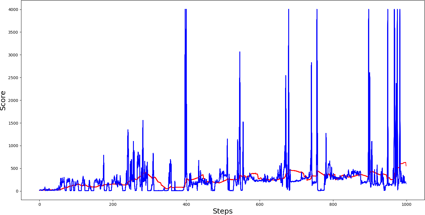
    #agent.test()

A comparison of the training progress of the agent in the CartPole environment under Double DQN, Dueling DQN, and Double dueling DQN architectures can be observed in the figures below, with the x-axis being the number of episodes:

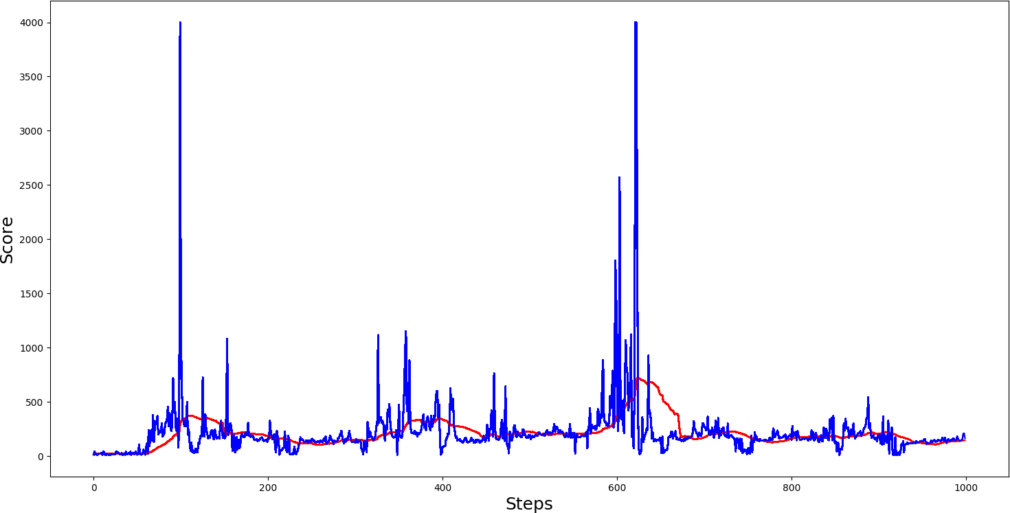
1. The first example is with a Single dueling DQN:

2. The second example is with Double DQN:

3. The third example is with Double dueling DQN:

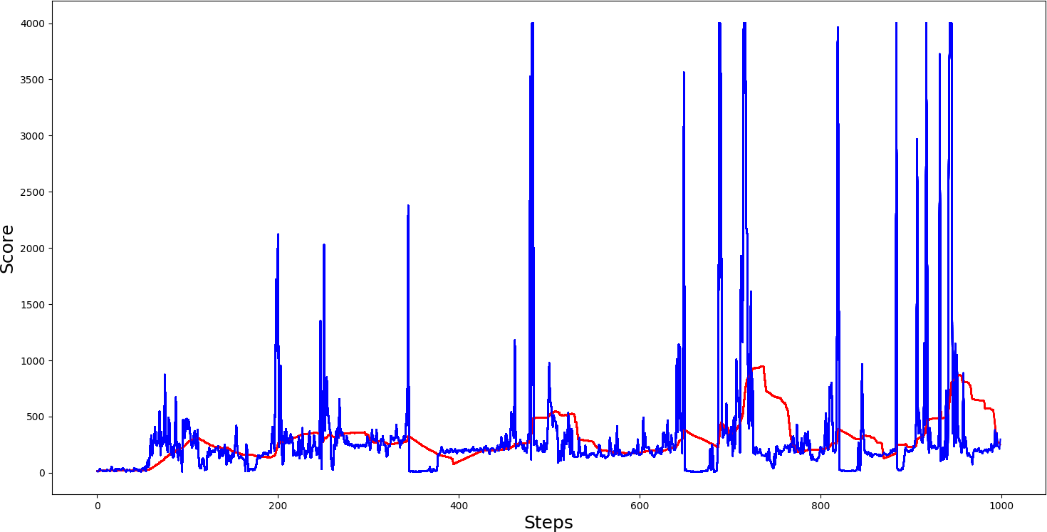The above graphs show that a single dueling cartpole isn't better than a single not dueling cartpole. The second example we made with DDQN architecture is getting comparable results with Dueling DDQN architecture. Seeing the graph, we can notice that we received much more maximum spikes, and if we saved the model on top of spikes while testing, we would receive quite nice results.

Conclusion:

As can be seen, there is a slightly higher performance of the Double Q network concerning the Dueling Q network. However, the performance difference is relatively small and may vary due to random network initialization. As such, in a reasonably simple environment like the CartPole environment, the benefits of the Dueling Q network over the Double Q network may not be realized. However, in more complex environments like Atari, the Dueling Q architecture will likely be superior to Double Q (the original Dueling Q paper has shown). So, in future tutorials, we will demonstrate the Dueling DQN architecture in Atari or other more complex environments.