Solving the Cartpole with Double Deep Q Network

Double Deep Q learning introduction

In the first tutorial, we used a simple method to train the Deep Q Neural Network model to play the CartPole balancing game. In this second reinforcement learning tutorial part, our task will be the same, but this time we'll make our environment use two (Double) Neural Networks to train our primary model. Adding to this, we'll implement a 'soft' parameters update function to this, and finally, we will compare the results we got with each method.

This post will go into the original structure of the DQN agent presented in this article. We will implement additional enhancements written in the article, and the results of testing the implementation in the CartPole v-1 environment will be presented. It is assumed that the reader has a basic familiarity with reinforcement or machine learning (finished reading 1st tutorial).

The Agent implemented in this tutorial follows the structure of the original DQN introduced in this paper but is closer to what is known as a Double DQN. An enhanced version of the original DQN was introduced nine months later, utilizing its internal Neural Networks slightly differently in its learning process. Technically the Agent implemented in this tutorial isn't really a DQN since our networks only contain a few layers (4) and so are not actually that "deep", but the distinguishing ideas of Deep Q Learning are still utilized.

An additional enhancement changing how the Agent's Neural Networks work with each other, known as "soft target network updates", introduced in another Deep Q Learning paper, will also be tested in this tutorial code.

From my previous tutorial, we already know the case of the CartPole game. The state is represented by four values — cart position, cart velocity, pole angle, and the velocity of the pole's tip — and the Agent can take one of two actions at every step — moving left or moving right.

Double Deep Q learning

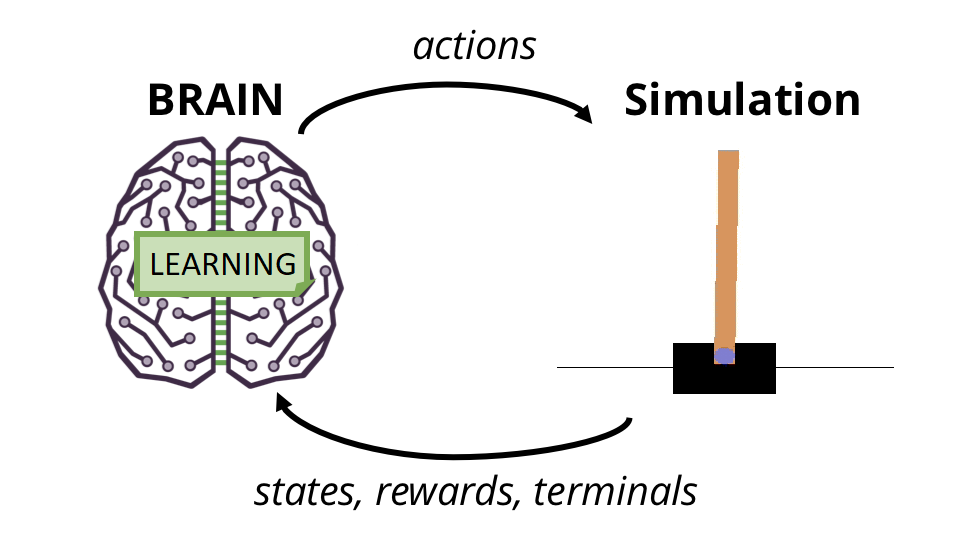
In Double Deep Q Learning, the Agent uses two neural networks to learn and predict what action to take at every step. One network, referred to as the Q network or the online network, predicts what to do when the Agent encounters a new state. It takes in the state as input and outputs Q values for the possible actions taken. In the Agent described in this tutorial, the online network takes in a vector of four values (state of the CartPole environment) as input. It outputs a vector of two Q values, one for the value of moving left in the current state and one for moving right in the current state. The Agent will choose the action that has the higher corresponding Q value output by the online network.

Double DQNs handle the problem of the overestimation of Q-values. We face a simple problem by calculating the target with the single deep network: we decide the best future state action with the highest Q-value.

From the first tutorial, we know that the accuracy of Q values depends on historical actions we tried and what neighboring states we explored.

Consequently, we don't have enough information about the best action to take at the beginning of the training. Therefore, taking the maximum q value (which is noisy) as the best action to take can lead to false positives. If non-optimal actions are regularly given a higher Q value than the optimal best action, the learning will be complicated.

The solution is: when we compute the Q target, we use two networks to decouple the action selected from the target Q value generation. We:

• Use our DQN network to choose what is the best action to take for the following state (the action with the highest Q value);
• Use our target network to calculate the target Q value of taking that action at the next state.

Therefore, Double DQN helps us reduce the overestimation of Q values and allows us to train faster and have more stable learning.

To understand Double DQN, let's analyze practical examples with a path of the Agent through different states. The process of Double Q-Learning can be visualized in the following graph:

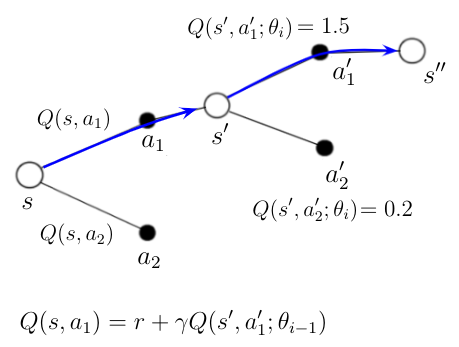An AI agent is at the start in state s. Agent, based on some previous calculations, knows the qualities Q(s, a1) and Q(s, a2) for possible two actions in that state. The agent decides to take action a1 and ends up in a state s’.

The Q-Network calculates the qualities Q(s’, a1') and Q(s, a2') for possible actions in this new state. Action a1' is picked because it results in the highest quality according to the Q-Network.

The new action-value Q(s, a1) for action a1 in the state s can now be calculated with the equation in the above figure, where Q(s’,a1') is the evaluation of a1' that is determined by the Target-Network.

Double Deep Q learning

All DQN agents learn and improve themselves through a method called experience replay, which is where in Double DQN, the second network, called the target network, comes into play. To carry out experience replay, the agent “remembers” each step of the game after it happens, each memory consisting of the action taken, the state that was in place when the action was taken, the reward given from taking action, and the state that resulted from taking action. These memories are also known as experiences. After each step is taken in the episode, the experience replay procedure is carried out (after enough memories have been stored) and consists of the following steps:

• a random set of experiences (called a minibatch) is retrieved from the agent’s memory;
• for each experience in the minibatch, new Q values are calculated for each state and action pair — if the action ended the episode, the Q value would be negative (bad). If the action did not end the game (i.e., kept the agent alive for at least one more turn), the Q value will be positive and is predicted by a Bellman equation. The general formula of the Bellman equation used by the agent implemented here is:

  value = reward + discount_factor * target_network.predict(next_state)[argmax(online_network.predict(next_state))]

• the NN is fit to associate each state in the minibatch with the new Q values calculated for the actions taken.

Below is the experience replay method used in code with short explanations:

def replay(self):
    if len(self.memory) < self.train_start:
        return
    # Randomly sample minibatch from the memory
    minibatch = random.sample(self.memory, min(self.batch_size, self.batch_size))

    state = np.zeros((self.batch_size, self.state_size))
    next_state = np.zeros((self.batch_size, self.state_size))
    action, reward, done = [], [], []

    # do this before prediction
    # for speedup, this could be done on the tensor level
    # but easier to understand using a loop
    for i in range(self.batch_size):
        state[i] = minibatch[i][0]
        action.append(minibatch[i][1])
        reward.append(minibatch[i][2])
        next_state[i] = minibatch[i][3]
        done.append(minibatch[i][4])

    # do batch prediction to save speed
    target = self.model.predict(state)
    target_next = self.model.predict(next_state)
    target_val = self.target_model.predict(next_state)

    for i in range(len(minibatch)):
        # correction on the Q value for the action used
        if done[i]:
            target[i][action[i]] = reward[i]
        else:
            if self.ddqn: # Double - DQN
                # current Q Network selects the action
                # a'_max = argmax_a' Q(s', a')
                a = np.argmax(target_next[i])
                # target Q Network evaluates the action
                # Q_max = Q_target(s', a'_max)
                target[i][action[i]] = reward[i] + self.gamma * (target_val[i][a])   
            else: # Standard - DQN
                # DQN chooses the max Q value among next actions
                # selection and evaluation of action is on the target Q Network
                # Q_max = max_a' Q_target(s', a')
                target[i][action[i]] = reward[i] + self.gamma * (np.amax(target_next[i]))

    # Train the Neural Network with batches
    self.model.fit(state, target, batch_size=self.batch_size, verbose=0)

Why are two networks needed to generate the new Q value for each action? The single online network could be used to generate the Q value to update. Still, if it did, then each update would consist of the single online network updating its weights to predict better what it itself outputs — the agent is trying to fit a target value that it itself defines and this can result in the network quickly updating itself too drastically in an unproductive way. To avoid this situation, the Q values to update are taken from the output of the second target network, which is meant to reflect the state of the online network but does not hold identical values.

From the above code, you can see that there is a line if self.ddqn:The code is written so that we would need to change one defined variable to False, and we'll be using standard DQN; this will help us compare different results of these models.

What makes this network a Double DQN?

The Bellman equation used to calculate the Q values to update the online network follows the equation:

value = reward + discount_factor * target_network.predict(next_state)[argmax(online_network.predict(next_state))]

The Bellman equation used to calculate the Q value updates in the original DQN is:

value = reward + discount_factor * max(target_network.predict(next_state))

The difference is that using the field terminology, the second equation uses the target network for both SELECTING and EVALUATING the action. In contrast, the first equation uses the online network for SELECTING the action and the target network for EVALUATING the action. The selection here means choosing which action to take, and evaluation means getting the projected Q value for that action. This form of the Bellman equation makes this agent a Double DQN and not just a DQN.

Soft Target Network Update

The method used to update the target network’s weights in the original DQN paper is to set them equal to the weights of the online network for every fixed number of steps. Another established method introduced here suggests updating the target network weights incrementally. This means that our target network weights should reflect the online network weights after every run of experience replay with the following formula:
target_weights = target_weights * (1-TAU) + q_weights * TAU where 0 < TAU < 1

def update_target_model(self):
    if not self.Soft_Update and self.ddqn:
        self.target_model.set_weights(self.model.get_weights())
        return
    if self.Soft_Update and self.ddqn:
        q_model_theta = self.model.get_weights()
        target_model_theta = self.target_model.get_weights()
        counter = 0
        for q_weight, target_weight in zip(q_model_theta, target_model_theta):
            target_weight = target_weight * (1-self.TAU) + q_weight * self.TAU
            target_model_theta[counter] = target_weight
            counter += 1
        self.target_model.set_weights(target_model_theta)

If you don't understand code here, don't worry. It's much easier to understand everything when you get deeper into full code. But simply talking, if we would use TAU as 0.1, then we would get the result as target_weights=target_weights*0.9+q_weights*0.1. This means that we are updating only 10% of new weights, using 90% of old weights.

Summary:

By running through experience replay every time the agent takes action and updating the parameters of the online network, the online network will begin to associate certain state/action pairs with appropriate Q values — the greater promise there is for taking a certain action at a certain state, the model will begin to predict higher Q values, and will start to survive for as long as the agent keeps playing the game.

So in full code implementations, we wrote few simple functions to track our scores and plot results in graphs for better visual comparison. Here are the following functions:

pylab.figure(figsize=(18, 9))
def PlotModel(self, score, episode):
    self.scores.append(score)
    self.episodes.append(episode)
    self.average.append(sum(self.scores) / len(self.scores))
    pylab.plot(self.episodes, self.average, 'r')
    pylab.plot(self.episodes, self.scores, 'b')
    pylab.ylabel('Score', fontsize=18)
    pylab.xlabel('Steps', fontsize=18)
    dqn = 'DQN_'
    softupdate = ''
    if self.ddqn:
        dqn = 'DDQN_'
    if self.Soft_Update:
        softupdate = '_soft'
    try:
        pylab.savefig(dqn+self.env_name+softupdate+".png")
    except OSError:
        pass

    return str(self.average[-1])[:5]

At the end of this tutorial is full code. With this code, we did 3 different experiments, where:
1. self.Soft_Update = False and self.ddqn = False;
2. self.Soft_Update = False and self.ddqn = True;
3. self.Soft_Update = True and self.ddqn = True.

That our experiment would not be too long, we defined maximum episode steps to train as 1000: self.EPISODES = 1000.

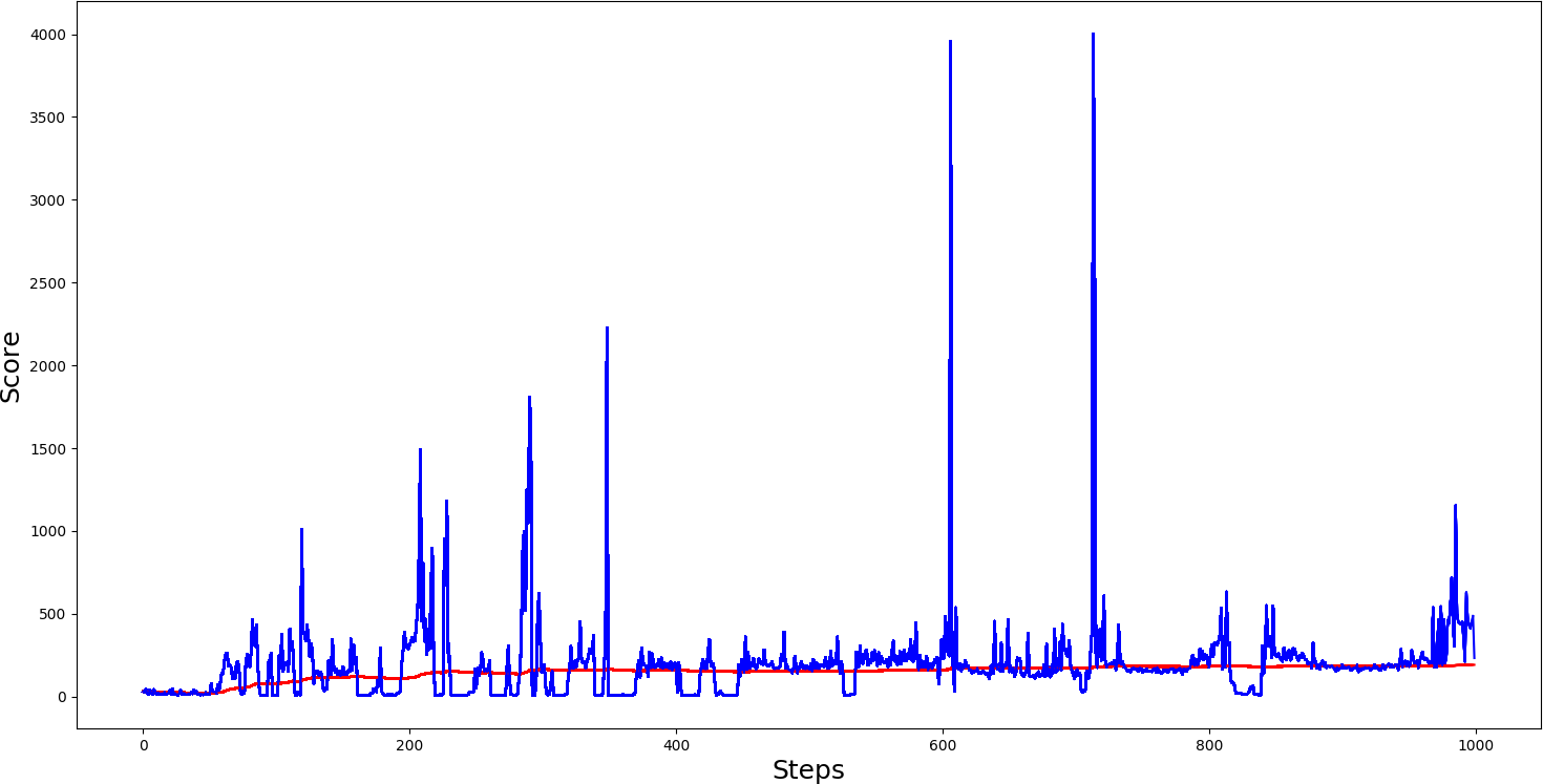
The first test was: with self.Soft_Update = False and self.ddqn = False, so with these parameters, we were using a standard DQN network without a soft update. From the following graph results, we can see that learning wasn't stable, and we were always receiving random spikes, but if we tried this model in test mode, it would perform the same way (constant low results with spikes) but our goal is stable solving.

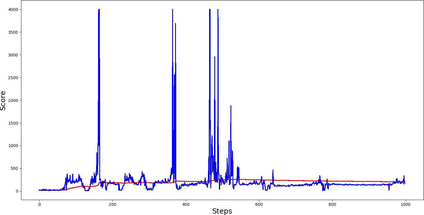
The third test was with self.Soft_Update = True and self.ddqn = True, so with these parameters, we were using a Double DQN network with a soft update. The following graph shows that results look quite the same as not using soft update, so it's quite hard to say if it has some effect. To get better results, maybe it would be better to do more tests.

# Tutorial by www.pylessons.com
# Tutorial written for - Tensorflow 1.15, Keras 2.2.4

import os
import random
import gym
import pylab
import numpy as np
from collections import deque
from keras.models import Model, load_model
from keras.layers import Input, Dense
from keras.optimizers import Adam, RMSprop

def OurModel(input_shape, action_space):
    X_input = Input(input_shape)
    X = X_input

    # 'Dense' is the basic form of a neural network layer
    # Input Layer of state size(4) and Hidden Layer with 512 nodes
    X = Dense(512, input_shape=input_shape, activation="relu", kernel_initializer='he_uniform')(X)

    # Hidden layer with 256 nodes
    X = Dense(256, activation="relu", kernel_initializer='he_uniform')(X)
    
    # Hidden layer with 64 nodes
    X = Dense(64, activation="relu", kernel_initializer='he_uniform')(X)

    # Output Layer with # of actions: 2 nodes (left, right)
    X = Dense(action_space, activation="linear", kernel_initializer='he_uniform')(X)

    model = Model(inputs = X_input, outputs = X, name='CartPole DDQN model')
    model.compile(loss="mean_squared_error", optimizer=RMSprop(lr=0.00025, rho=0.95, epsilon=0.01), metrics=["accuracy"])

    model.summary()
    return model

class DQNAgent:
    def __init__(self, env_name):
        self.env_name = env_name       
        self.env = gym.make(env_name)
        self.env.seed(0)  
        # by default, CartPole-v1 has max episode steps = 500
        self.env._max_episode_steps = 4000
        self.state_size = self.env.observation_space.shape[0]
        self.action_size = self.env.action_space.n

        self.EPISODES = 1000
        self.memory = deque(maxlen=2000)
        
        self.gamma = 0.95    # discount rate
        self.epsilon = 1.0  # exploration rate
        self.epsilon_min = 0.01
        self.epsilon_decay = 0.999
        self.batch_size = 32
        self.train_start = 1000

        # defining model parameters
        self.ddqn = True
        self.Soft_Update = False

        self.TAU = 0.1 # target network soft update hyperparameter

        self.Save_Path = 'Models'
        self.scores, self.episodes, self.average = [], [], []
        
        if self.ddqn:
            print("----------Double DQN--------")
            self.Model_name = os.path.join(self.Save_Path,"DDQN_"+self.env_name+".h5")
        else:
            print("-------------DQN------------")
            self.Model_name = os.path.join(self.Save_Path,"DQN_"+self.env_name+".h5")
        
        # create main model
        self.model = OurModel(input_shape=(self.state_size,), action_space = self.action_size)
        self.target_model = OurModel(input_shape=(self.state_size,), action_space = self.action_size)

    # after some time interval update the target model to be same with model
    def update_target_model(self):
        if not self.Soft_Update and self.ddqn:
            self.target_model.set_weights(self.model.get_weights())
            return
        if self.Soft_Update and self.ddqn:
            q_model_theta = self.model.get_weights()
            target_model_theta = self.target_model.get_weights()
            counter = 0
            for q_weight, target_weight in zip(q_model_theta, target_model_theta):
                target_weight = target_weight * (1-self.TAU) + q_weight * self.TAU
                target_model_theta[counter] = target_weight
                counter += 1
            self.target_model.set_weights(target_model_theta)

    def remember(self, state, action, reward, next_state, done):
        self.memory.append((state, action, reward, next_state, done))
        if len(self.memory) > self.train_start:
            if self.epsilon > self.epsilon_min:
                self.epsilon *= self.epsilon_decay

    def act(self, state):
        if np.random.random() <= self.epsilon:
            return random.randrange(self.action_size)
        else:
            return np.argmax(self.model.predict(state))

    def replay(self):
        if len(self.memory) < self.train_start:
            return
        # Randomly sample minibatch from the memory
        minibatch = random.sample(self.memory, min(self.batch_size, self.batch_size))

        state = np.zeros((self.batch_size, self.state_size))
        next_state = np.zeros((self.batch_size, self.state_size))
        action, reward, done = [], [], []

        # do this before prediction
        # for speedup, this could be done on the tensor level
        # but easier to understand using a loop
        for i in range(self.batch_size):
            state[i] = minibatch[i][0]
            action.append(minibatch[i][1])
            reward.append(minibatch[i][2])
            next_state[i] = minibatch[i][3]
            done.append(minibatch[i][4])

        # do batch prediction to save speed
        target = self.model.predict(state)
        target_next = self.model.predict(next_state)
        target_val = self.target_model.predict(next_state)

        for i in range(len(minibatch)):
            # correction on the Q value for the action used
            if done[i]:
                target[i][action[i]] = reward[i]
            else:
                if self.ddqn: # Double - DQN
                    # current Q Network selects the action
                    # a'_max = argmax_a' Q(s', a')
                    a = np.argmax(target_next[i])
                    # target Q Network evaluates the action
                    # Q_max = Q_target(s', a'_max)
                    target[i][action[i]] = reward[i] + self.gamma * (target_val[i][a])   
                else: # Standard - DQN
                    # DQN chooses the max Q value among next actions
                    # selection and evaluation of action is on the target Q Network
                    # Q_max = max_a' Q_target(s', a')
                    target[i][action[i]] = reward[i] + self.gamma * (np.amax(target_next[i]))

        # Train the Neural Network with batches
        self.model.fit(state, target, batch_size=self.batch_size, verbose=0)


    def load(self, name):
        self.model = load_model(name)

    def save(self, name):
        self.model.save(name)

    pylab.figure(figsize=(18, 9))
    def PlotModel(self, score, episode):
        self.scores.append(score)
        self.episodes.append(episode)
        self.average.append(sum(self.scores) / len(self.scores))
        pylab.plot(self.episodes, self.average, 'r')
        pylab.plot(self.episodes, self.scores, 'b')
        pylab.ylabel('Score', fontsize=18)
        pylab.xlabel('Steps', fontsize=18)
        dqn = 'DQN_'
        softupdate = ''
        if self.ddqn:
            dqn = 'DDQN_'
        if self.Soft_Update:
            softupdate = '_soft'
        try:
            pylab.savefig(dqn+self.env_name+softupdate+".png")
        except OSError:
            pass

        return str(self.average[-1])[:5]
    
    def run(self):
        for e in range(self.EPISODES):
            state = self.env.reset()
            state = np.reshape(state, [1, self.state_size])
            done = False
            i = 0
            while not done:
                #self.env.render()
                action = self.act(state)
                next_state, reward, done, _ = self.env.step(action)
                next_state = np.reshape(next_state, [1, self.state_size])
                if not done or i == self.env._max_episode_steps-1:
                    reward = reward
                else:
                    reward = -100
                self.remember(state, action, reward, next_state, done)
                state = next_state
                i += 1
                if done:
                    # every step update target model
                    self.update_target_model()
                    
                    # every episode, plot the result
                    average = self.PlotModel(i, e)
                     
                    print("episode: {}/{}, score: {}, e: {:.2}, average: {}".format(e, self.EPISODES, i, self.epsilon, average))
                    if i == self.env._max_episode_steps:
                        print("Saving trained model as cartpole-ddqn.h5")
                        #self.save("cartpole-ddqn.h5")
                        break
                self.replay()

    def test(self):
        self.load("cartpole-ddqn.h5")
        for e in range(self.EPISODES):
            state = self.env.reset()
            state = np.reshape(state, [1, self.state_size])
            done = False
            i = 0
            while not done:
                self.env.render()
                action = np.argmax(self.model.predict(state))
                next_state, reward, done, _ = self.env.step(action)
                state = np.reshape(next_state, [1, self.state_size])
                i += 1
                if done:
                    print("episode: {}/{}, score: {}".format(e, self.EPISODES, i))
                    break

if __name__ == "__main__":
    env_name = 'CartPole-v1'
    agent = DQNAgent(env_name)
    agent.run()
    #agent.test()

Conclusion:

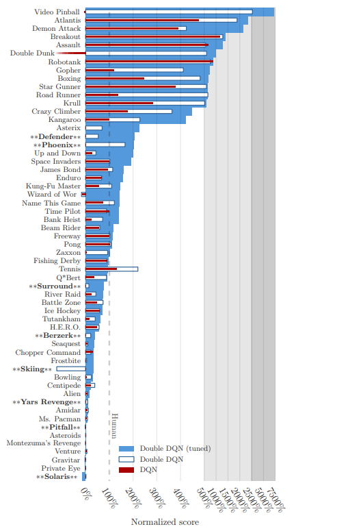
This tutorial goal was to test the Double DQN agent and test the received results. However, from one test, we can't say that Double DQN is much better than DQN, but knowing that David Silver et al. tested Deep Q-Networks (DQNs) and Deep Double Q-Networks (Double DQNs) on several Atari 2600 games. The normalized scores achieved by AI agents of those two methods and comparable human performance are shown below. The figure also contains a tuned version of Double DQN where some hyper-parameter optimization was performed.

It can be clearly noticed that these two different versions of Double DQNs achieve better performances in this area than their vanilla implementation. The code for this tutorial can be found on the GitHub link.