Since the beginning of this Reinforcement Learning tutorial series, I've covered two different reinforcement learning methods: Value-based methods (Q-learning, Deep Q-learning…) and Policy-based methods (REINFORCE with Policy Gradients).
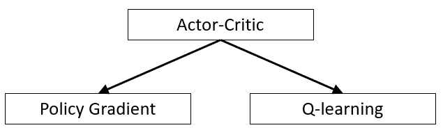
Both of these methods have considerable drawbacks. That's why, today, I'll try another type of Reinforcement Learning method, which we can call a 'hybrid method': Actor-Critic. The actor-Critic algorithm is a Reinforcement Learning agent that combines value optimization and policy optimization approaches. More specifically, the Actor-Critic combines the Q-learning and Policy Gradient algorithms. The resulting algorithm obtained at the high level involves a cycle that shares features between:
- Actor: a PG algorithm that decides on an action to take;
- Critic: Q-learning algorithm that critiques the action that the Actor selected, providing feedback on how to adjust. It can take advantage of efficiency tricks in Q-learning, such as memory replay.
The advantage of the Actor-Critic algorithm is that it can solve a broader range of problems than DQN, while it has a lower variance in performance relative to REINFORCE. That said, because of the presence of the PG algorithm within it, the Actor-Critic is still somewhat sampling inefficient.
The problem with Policy Gradients:
In my previous tutorial, we derived policy gradients and implemented the REINFORCE algorithm (also known as Monte Carlo policy gradients). There are, however, some issues with vanilla policy gradients: noisy gradients and high variance.
Recall the policy gradient function:
The REINFORCE algorithm updates the policy parameter through Monte Carlo updates (i.e., taking random samples). This introduces inherent high variability in log probabilities (log of the policy distribution) and cumulative reward values because each training trajectory can deviate from each other to great degrees. Consequently, the high variability in log probabilities and cumulative reward values will make noisy gradients and cause unstable learning and/or the policy distribution skewing to a non-optimal direction. Besides high variance of gradients, another problem with policy gradients occurs trajectories have a cumulative reward of 0. The essence of policy gradient is to increase the probabilities for "good" actions and decrease those of "bad" actions in the policy distribution; both good and bad actions will not be learned if the cumulative reward is 0. Overall, these issues contribute to the instability and slow convergence of vanilla policy gradient methods. One way to reduce variance and increase stability is subtracting the cumulative reward by a baseline b(s):
Intuitively, making the cumulative reward smaller by subtracting it with a baseline will make smaller gradients and thus more minor and more stable updates.
How Actor-Critic works:
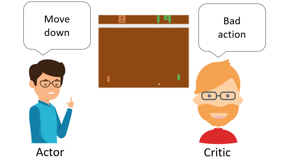
Imagine you play a video game with a friend that provides you some feedback. You're the Actor, and your friend is the Critic:
 In the beginning, you don't know how to play, so you try some action randomly. The Critic observes your action and provides feedback. Let's first take a look at the vanilla policy gradient again to see how the Actor-Critic architecture comes in (and what it is):
We can then decompose the expectation into:
The second expectation term should be familiar; it is the Q value!
Plugging that in, we can rewrite the update equation as such:
As we know, the Q value can be learned by parameterizing the Q function with a neural network. This leads us to Actor-Critic Methods, where:
- The "Critic" estimates the value function. This could be the action-value (the Q value) or state-value (the V value).
- Critic: Q-learning algorithm that critiques the action that the Actor selected, providing feedback on how to adjust. It can take advantage of efficiency tricks in Q-learning, such as memory replay.
We update both the Critic network and the Value network at each update step.
Intuitively, this means how better it is to take a specific action than the average general action at the given state. So, using the Value function as the baseline function, we subtract the Q value term with the Value. We will call this Value the advantage value:
This is so-called the Advantage Actor-Critic; in code, it looks much more straightforward, you will see.
Advantage Actor-Critic implementation:
I am working on my previous tutorial code; we need to add the Critic model to the same principle. So in Policy Gradient, our model looked following:
def OurModel(input_shape, action_space, lr):
    X_input = Input(input_shape)

    X = Flatten(input_shape=input_shape)(X_input)

    X = Dense(512, activation="elu", kernel_initializer='he_uniform')(X)

    action = Dense(action_space, activation="softmax", kernel_initializer='he_uniform')(X)

    Actor = Model(inputs = X_input, outputs = action)
    Actor.compile(loss='categorical_crossentropy', optimizer=RMSprop(lr=lr))

    return Actor
To make it Actor-Critic, we add the 'value' parameter, and we compile not only the Actor model but and Critic model with 'mse' loss:
def OurModel(input_shape, action_space, lr):
    X_input = Input(input_shape)

    X = Flatten(input_shape=input_shape)(X_input)

    X = Dense(512, activation="elu", kernel_initializer='he_uniform')(X)

    action = Dense(action_space, activation="softmax", kernel_initializer='he_uniform')(X)
    value = Dense(1, kernel_initializer='he_uniform')(X)

    Actor = Model(inputs = X_input, outputs = action)
    Actor.compile(loss='categorical_crossentropy', optimizer=RMSprop(lr=lr))

    Critic = Model(inputs = X_input, outputs = value)
    Critic.compile(loss='mse', optimizer=RMSprop(lr=lr))

    return Actor, Critic
Another most important function we change is a def replay(self). In policy gradient, it looked following:
def replay(self):
    # reshape memory to appropriate shape for training
    states = np.vstack(self.states)
    actions = np.vstack(self.actions)

    # Compute discounted rewards
    discounted_r = self.discount_rewards(self.rewards)

    # training PG network
    self.Actor.fit(states, actions, sample_weight=discounted_r, epochs=1, verbose=0)
    # reset training memory
    self.states, self.actions, self.rewards = [], [], []
To make it work as an Actor-Critic algorithm, we predict states without the Critic model to get values that we subtract from discounted rewards, and this is how we calculate advantages. And instead of training Actor with discounted rewards, we use advantages, and for the Critic network, we use discounted rewards:
def replay(self):
    # reshape memory to appropriate shape for training
    states = np.vstack(self.states)
    actions = np.vstack(self.actions)

    # Compute discounted rewards
    discounted_r = self.discount_rewards(self.rewards)

    # Get Critic network predictions
    values = self.Critic.predict(states)[:, 0]
    # Compute advantages
    advantages = discounted_r - values
    # training Actor and Critic networks
    self.Actor.fit(states, actions, sample_weight=advantages, epochs=1, verbose=0)
    self.Critic.fit(states, discounted_r, epochs=1, verbose=0)
    # reset training memory
    self.states, self.actions, self.rewards = [], [], []
That's it; we just needed to change few lines of code. Moreover, you can change the 'save' and 'load model' functions. Here is the complete code:
# Tutorial by www.pylessons.com
# Tutorial written for - Tensorflow 1.15, Keras 2.2.4

import os
import random
import gym
import pylab
import numpy as np
from keras.models import Model, load_model
from keras.layers import Input, Dense, Lambda, Add, Conv2D, Flatten
from keras.optimizers import Adam, RMSprop
from keras import backend as K
import cv2

def OurModel(input_shape, action_space, lr):
    X_input = Input(input_shape)

    #X = Conv2D(32, 8, strides=(4, 4),padding="valid", activation="elu", data_format="channels_first", input_shape=input_shape)(X_input)
    #X = Conv2D(64, 4, strides=(2, 2),padding="valid", activation="elu", data_format="channels_first")(X)
    #X = Conv2D(64, 3, strides=(1, 1),padding="valid", activation="elu", data_format="channels_first")(X)
    X = Flatten(input_shape=input_shape)(X_input)

    X = Dense(512, activation="elu", kernel_initializer='he_uniform')(X)
    #X = Dense(256, activation="elu", kernel_initializer='he_uniform')(X)
    #X = Dense(64, activation="elu", kernel_initializer='he_uniform')(X)

    action = Dense(action_space, activation="softmax", kernel_initializer='he_uniform')(X)
    value = Dense(1, kernel_initializer='he_uniform')(X)

    Actor = Model(inputs = X_input, outputs = action)
    Actor.compile(loss='categorical_crossentropy', optimizer=RMSprop(lr=lr))

    Critic = Model(inputs = X_input, outputs = value)
    Critic.compile(loss='mse', optimizer=RMSprop(lr=lr))

    return Actor, Critic

class A2CAgent:
    # Actor-Critic Main Optimization Algorithm
    def __init__(self, env_name):
        # Initialization
        # Environment and PPO parameters
        self.env_name = env_name
        self.env = gym.make(env_name)
        self.action_size = self.env.action_space.n
        self.EPISODES, self.max_average = 10000, -21.0 # specific for pong
        self.lr = 0.000025

        self.ROWS = 80
        self.COLS = 80
        self.REM_STEP = 4

        # Instantiate games and plot memory
        self.states, self.actions, self.rewards = [], [], []
        self.scores, self.episodes, self.average = [], [], []

        self.Save_Path = 'Models'
        self.state_size = (self.REM_STEP, self.ROWS, self.COLS)
        self.image_memory = np.zeros(self.state_size)

        if not os.path.exists(self.Save_Path): os.makedirs(self.Save_Path)
        self.path = '{}_A2C_{}'.format(self.env_name, self.lr)
        self.Model_name = os.path.join(self.Save_Path, self.path)

        # Create Actor-Critic network model
        self.Actor, self.Critic = OurModel(input_shape=self.state_size, action_space = self.action_size, lr=self.lr)


    def remember(self, state, action, reward):
        # store episode actions to memory
        self.states.append(state)
        action_onehot = np.zeros([self.action_size])
        action_onehot[action] = 1
        self.actions.append(action_onehot)
        self.rewards.append(reward)


    def act(self, state):
        # Use the network to predict the next action to take, using the model
        prediction = self.Actor.predict(state)[0]
        action = np.random.choice(self.action_size, p=prediction)
        return action

    def discount_rewards(self, reward):
        # Compute the gamma-discounted rewards over an episode
        gamma = 0.99    # discount rate
        running_add = 0
        discounted_r = np.zeros_like(reward)
        for i in reversed(range(0,len(reward))):
            if reward[i] != 0: # reset the sum, since this was a game boundary (pong specific!)
                running_add = 0
            running_add = running_add * gamma + reward[i]
            discounted_r[i] = running_add

        discounted_r -= np.mean(discounted_r) # normalizing the result
        discounted_r /= np.std(discounted_r) # divide by standard deviation
        return discounted_r


    def replay(self):
        # reshape memory to appropriate shape for training
        states = np.vstack(self.states)
        actions = np.vstack(self.actions)

        # Compute discounted rewards
        discounted_r = self.discount_rewards(self.rewards)

        # Get Critic network predictions
        values = self.Critic.predict(states)[:, 0]
        # Compute advantages
        advantages = discounted_r - values
        # training Actor and Critic networks
        self.Actor.fit(states, actions, sample_weight=advantages, epochs=1, verbose=0)
        self.Critic.fit(states, discounted_r, epochs=1, verbose=0)
        # reset training memory
        self.states, self.actions, self.rewards = [], [], []

    def load(self, Actor_name, Critic_name):
        self.Actor = load_model(Actor_name, compile=False)
        #self.Critic = load_model(Critic_name, compile=False)

    def save(self):
        self.Actor.save(self.Model_name + '_Actor.h5')
        #self.Critic.save(self.Model_name + '_Critic.h5')

    pylab.figure(figsize=(18, 9))
    def PlotModel(self, score, episode):
        self.scores.append(score)
        self.episodes.append(episode)
        self.average.append(sum(self.scores[-50:]) / len(self.scores[-50:]))
        if str(episode)[-2:] == "00":# much faster than episode % 100
            pylab.plot(self.episodes, self.scores, 'b')
            pylab.plot(self.episodes, self.average, 'r')
            pylab.ylabel('Score', fontsize=18)
            pylab.xlabel('Steps', fontsize=18)
            try:
                pylab.savefig(self.path+".png")
            except OSError:
                pass

        return self.average[-1]

    def imshow(self, image, rem_step=0):
        cv2.imshow(self.Model_name+str(rem_step), image[rem_step,...])
        if cv2.waitKey(25) & 0xFF == ord("q"):
            cv2.destroyAllWindows()
            return

    def GetImage(self, frame):
        # croping frame to 80x80 size
        frame_cropped = frame[35:195:2, ::2,:]
        if frame_cropped.shape[0] != self.COLS or frame_cropped.shape[1] != self.ROWS:
            # OpenCV resize function
            frame_cropped = cv2.resize(frame, (self.COLS, self.ROWS), interpolation=cv2.INTER_CUBIC)

        # converting to RGB (numpy way)
        frame_rgb = 0.299*frame_cropped[:,:,0] + 0.587*frame_cropped[:,:,1] + 0.114*frame_cropped[:,:,2]

        # convert everything to black and white (agent will train faster)
        frame_rgb[frame_rgb < 100] = 0
        frame_rgb[frame_rgb >= 100] = 255
        # converting to RGB (OpenCV way)
        #frame_rgb = cv2.cvtColor(frame_cropped, cv2.COLOR_RGB2GRAY)

        # dividing by 255 we expresses value to 0-1 representation
        new_frame = np.array(frame_rgb).astype(np.float32) / 255.0

        # push our data by 1 frame, similar as deq() function work
        self.image_memory = np.roll(self.image_memory, 1, axis = 0)

        # inserting new frame to free space
        self.image_memory[0,:,:] = new_frame

        # show image frame
        #self.imshow(self.image_memory,0)
        #self.imshow(self.image_memory,1)
        #self.imshow(self.image_memory,2)
        #self.imshow(self.image_memory,3)

        return np.expand_dims(self.image_memory, axis=0)

    def reset(self):
        frame = self.env.reset()
        for i in range(self.REM_STEP):
            state = self.GetImage(frame)
        return state

    def step(self, action):
        next_state, reward, done, info = self.env.step(action)
        next_state = self.GetImage(next_state)
        return next_state, reward, done, info

    def run(self):
        for e in range(self.EPISODES):
            state = self.reset()
            done, score, SAVING = False, 0, ''
            while not done:
                #self.env.render()
                # Actor picks an action
                action = self.act(state)
                # Retrieve new state, reward, and whether the state is terminal
                next_state, reward, done, _ = self.step(action)
                # Memorize (state, action, reward) for training
                self.remember(state, action, reward)
                # Update current state
                state = next_state
                score += reward
                if done:
                    average = self.PlotModel(score, e)
                    # saving best models
                    if average >= self.max_average:
                        self.max_average = average
                        self.save()
                        SAVING = "SAVING"
                    else:
                        SAVING = ""
                    print("episode: {}/{}, score: {}, average: {:.2f} {}".format(e, self.EPISODES, score, average, SAVING))

                    self.replay()
        # close environemnt when finish training
        self.env.close()

    def test(self, Actor_name, Critic_name):
        self.load(Actor_name, Critic_name)
        for e in range(100):
            state = self.reset()
            done = False
            score = 0
            while not done:
                action = np.argmax(self.Actor.predict(state))
                state, reward, done, _ = self.step(action)
                score += reward
                if done:
                    print("episode: {}/{}, score: {}".format(e, self.EPISODES, score))
                    break
        self.env.close()

if __name__ == "__main__":
    #env_name = 'PongDeterministic-v4'
    env_name = 'Pong-v0'
    agent = A2CAgent(env_name)
    agent.run()
    #agent.test('Pong-v0_A2C_2.5e-05_Actor.h5', '')
Same as in my previous tutorial, I first trained 'PongDeterministic-v4' for 1000 steps, results you can see in bellow graph:
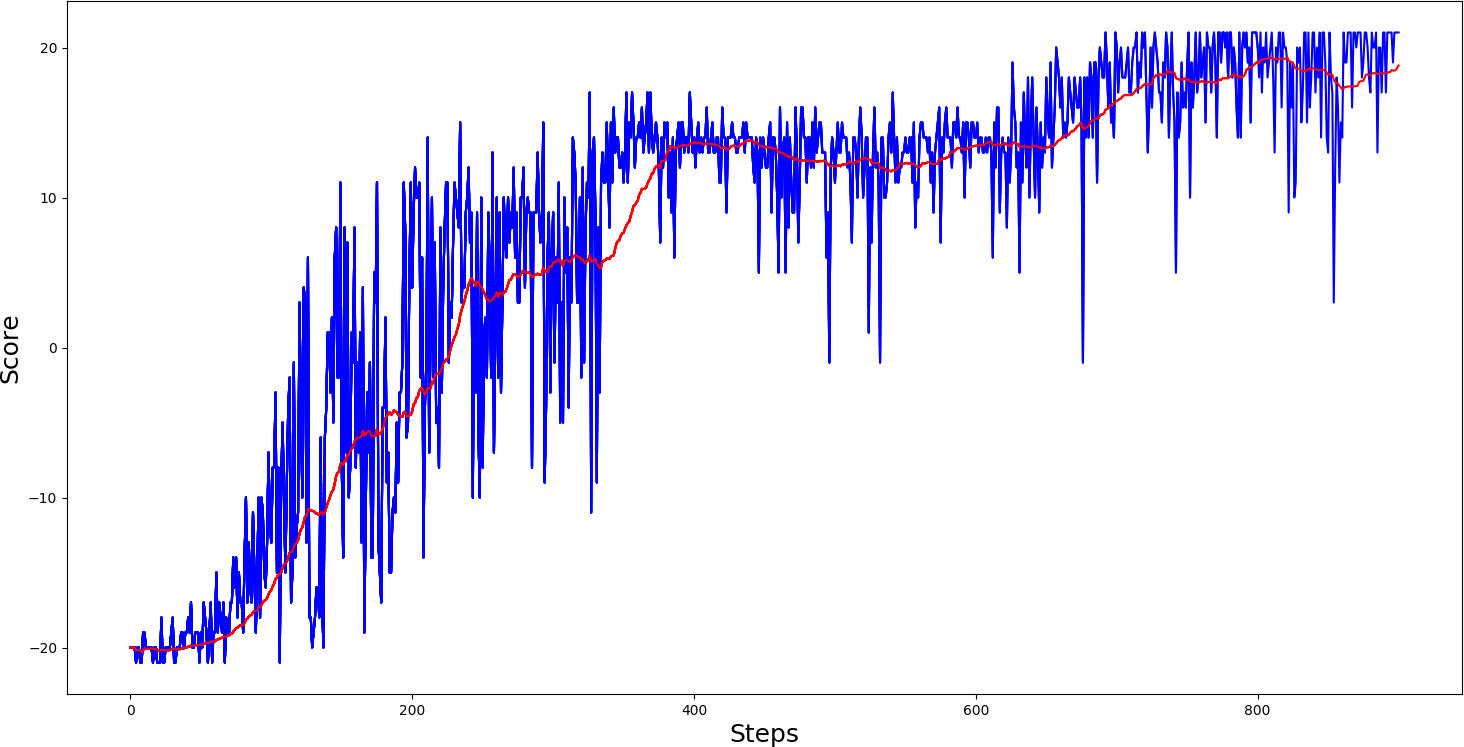 So, from the training results, we can say that the A2C model played pong relatively smoother. Despite that, it took a little longer to reach maximum scores, games of it were much more stable than PG, where we had many spikes. Then I thought, ok, let's give a chance to our 'Pong-v0' environment:
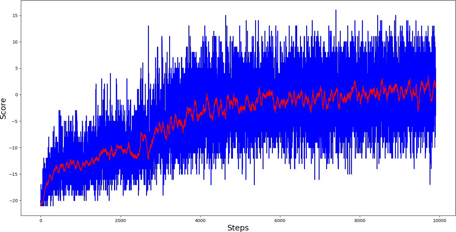
Now our 'Pong-v0' training graph looks much better than in Policy Gradient, much more stable games. But sadly, our average score couldn't get more than 11 scores per game. But keep in mind that I am using one deep layer network; you can play around with architecture.
Conclusion:
So, in this tutorial, we implemented a hybrid between value-based algorithms and policy-based algorithms. But we still face a problem, that learning for these models takes a lot of time. So in the next tutorial part, I will implement it as an Asynchronous A2C algorithm. This means that we will run, for example, four environments at once, and we will train the same main model. In theory, this means we will train our agent four times faster, but you will see how it looks in practice in the next tutorial part.