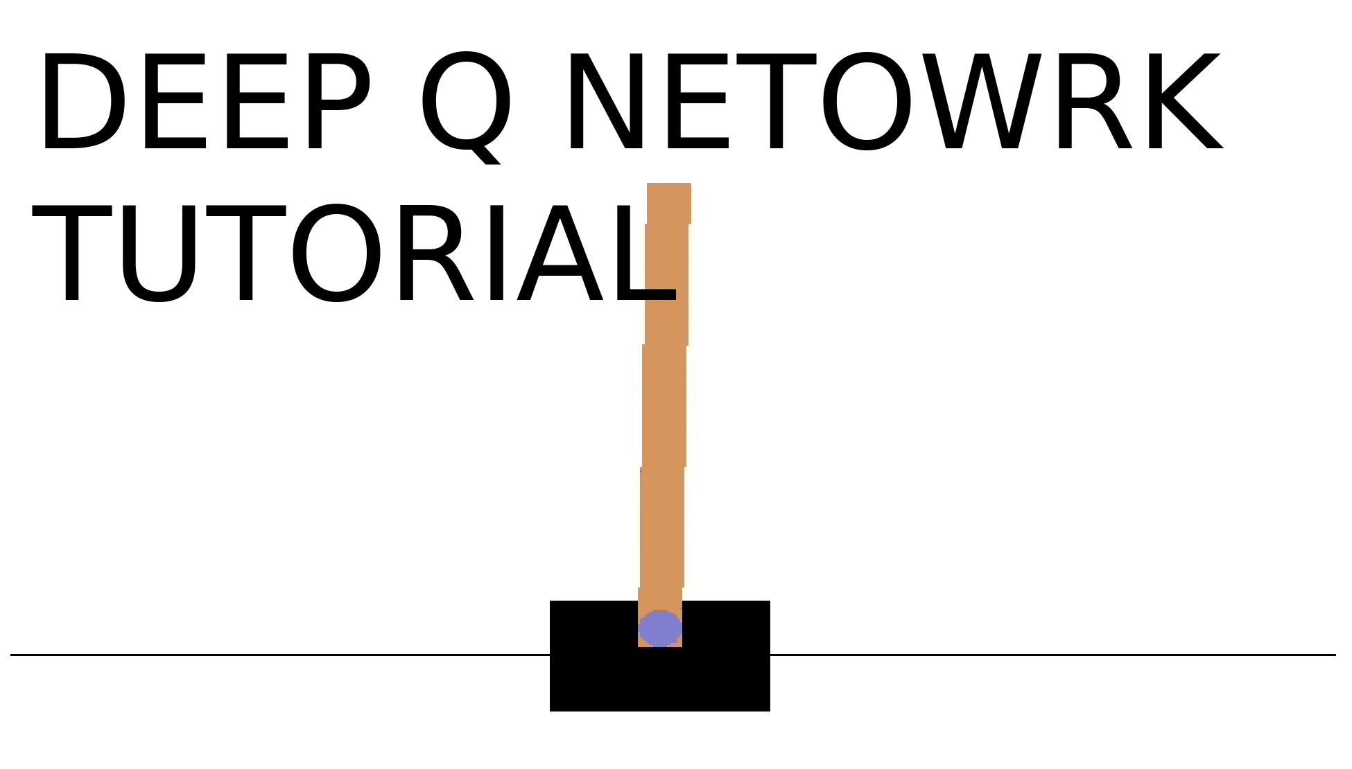
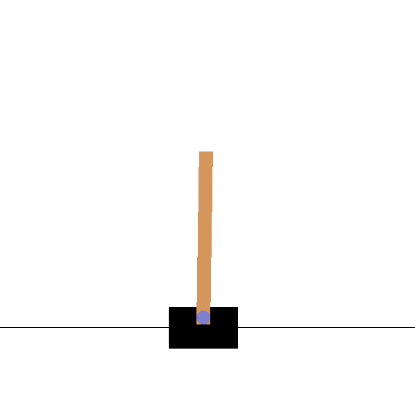
The idea of CartPole is that there is a pole standing up on top of a cart. The goal is to balance this pole by moving the cart from side to side to keep the stick balanced upright.
We consider the environment won if we balance it for 500 frames and fail once the pole is tilted more than 15 degrees from totally vertical or the cart moves more than 2.4 units from the middle position.
For every frame that we go with the pole "balanced" (less than 15 degrees from vertical), our "score" gets +1, and our target is a score of 500.
Now, however, how can we do this? There are countless ways in which we can do this. Some are very complex, and some are very specific to the environment. I chose to demonstrate how deep reinforcement learning (deep Q-learning) can be implemented and applied to play a CartPole game using Keras and Gym. I will try to explain everything without requiring any prerequisite knowledge about reinforcement learning.
Before starting, take a look at this YouTube video with a real-life demonstration of a CartPole problem learning process. Looks impressive, right? Implementing such a self-learning system is easier than you may think. Let's dive in!
Reinforcement Learning
To achieve the desired behavior of an agent that learns from its mistakes and improves its performance, we need to get more familiar with the concept of Reinforcement Learning (RL).
RL is a type of machine learning that allows us to create AI agents that learn from the environment by interacting with it to maximize its cumulative reward. In the same way, how we learn to ride a bicycle, AI learns it by trial and error, agents in RL algorithms are incentivized with punishments for wrong actions and rewards for good ones.
After each action, the agent receives feedback. The feedback consists of the reward and the next state of the environment. A human usually defines the reward. Using the bicycle analogy, we can define reward as the distance from the original starting point.
Cartpole Game
CartPole is one of the most straightforward environments in OpenAI gym (collection of environments to develop and test RL algorithms). Cartpole is built on a Markov chain model that I give illustration below.
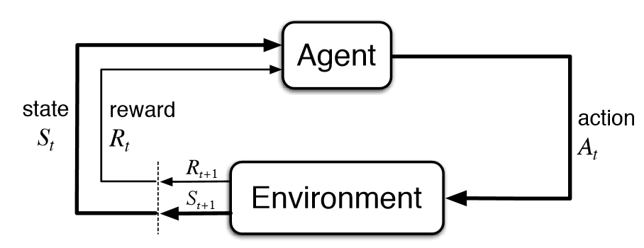
Then for each iteration, an agent takes the current state (St), picks the best (based on model prediction) action (At), and executes it on an environment. Subsequently, the environment returns a reward (Rt+1) for a given activity, a new state (St+1), and information if the new state is terminal. The process repeats until termination.
The goal of CartPole is to balance a pole connected with one joint on top of a moving cart. An agent can move the cart by performing a series of 0 or 1 actions, pushing it left or right. To simplify our task, instead of reading pixel information, there are four kinds of information given by the state: the angle of the pole and the cart's position.
The gym makes interacting with the game environment really simple:
next_state, reward, done, info = env.step(action)
Here, action can be either 0 or 1. If we pass those numbers, env, which represents the game environment, will emit the results. Done is a Boolean value telling whether the game ended or not. next_state space handles all possible state values:
(
[Cart Position from -4.8 to 4.8],
[Cart Velocity from -Inf to Inf],
[Pole Angle from -24° to 24°],
[Pole Velocity At Tip from -Inf to Inf]
)
The old state information paired with action, next_state, and reward is the information we need for training the agent.
So to understand everything from basics, lets first create a CartPole environment where our python script would play with it randomly:
import gym
import random

env = gym.make("CartPole-v1")

def Random_games():
    # Each of this episode is its own game.
    for episode in range(10):
        env.reset()
        # this is each frame, up to 500...but we wont make it that far with random.
        for t in range(500):
            # This will display the environment
            # Only display if you really want to see it.
            # Takes much longer to display it.
            env.render()

            # This will just create a sample action in any environment.
            # In this environment, the action can be 0 or 1, which is left or right
            action = env.action_space.sample()

            # this executes the environment with an action,
            # and returns the observation of the environment,
            # the reward, if the env is over, and other info.
            next_state, reward, done, info = env.step(action)

            # lets print everything in one line:
            print(t, next_state, reward, done, info, action)
            if done:
                break

Random_games()
Learn with Simple Neural Network using Keras
This tutorial is not about deep learning or neural networks. So I will not explain how it works in detail; I'll consider it just as a black-box algorithm that approximately maps inputs to outputs. That's a Neural Networks algorithm that learns on the pairs of examples input and output data, detect some patterns, and predicts the outcome based on unseen input data.
Neural networks are not the focus of this tutorial, but we should understand how it's used to learn in deep Q-learning algorithms.
Keras makes it simple to implement a basic neural network. With the code below, we will create an empty NN model. Activation, loss, and optimizer are the parameters that define the characteristics of the neural network, but we are not going to discuss them here.
from keras.models import Model
from keras.layers import Input, Dense
from keras.optimizers import Adam, RMSprop

# Neural Network model for Deep Q Learning
def OurModel(input_shape, action_space):
    X_input = Input(input_shape)

    # 'Dense' is the basic form of a neural network layer
    # Input Layer of state size(4) and Hidden Layer with 512 nodes
    X = Dense(512, input_shape=input_shape, activation="relu", kernel_initializer='he_uniform')(X_input)

    # Hidden layer with 256 nodes
    X = Dense(256, activation="relu", kernel_initializer='he_uniform')(X)

    # Hidden layer with 64 nodes
    X = Dense(64, activation="relu", kernel_initializer='he_uniform')(X)

    # Output Layer with # of actions: 2 nodes (left, right)
    X = Dense(action_space, activation="linear", kernel_initializer='he_uniform')(X)

    model = Model(inputs = X_input, outputs = X, name='CartPole DQN model')
    model.compile(loss="mse", optimizer=RMSprop(lr=0.00025, rho=0.95, epsilon=0.01), metrics=["accuracy"])

    model.summary()
    return model
For a NN to understand and predict based on the environment data, we have initialized our model (will show it in original code) and feed it to the information. Then the model will train on those data to approximate the output based on the input. Later in the complete code, you will see that the fit() method provides input and output pairs to the model.
In the above model, I used three layers of Neural Network, 512, 256, and 64 neurons. Feel free to play with its structure and parameters.
Later in the training process, you will see what makes the NN predict the reward value from a particular state. You will see that in code, I will use model.fit(next_state, reward), same as in the standard Keras NN model.
After training, the model we will be able to predict the output from unseen input. When we call predict() function on the model, the model will predict the reward of the current state based on the data we trained. Like so: prediction = model.predict(next_state)
Implementing Deep Q Network (DQN)
Generally, in games, the reward directly relates to the score of the game. But, imagine a situation where the pole from the CartPole game is tilted to the left. The expected future reward of pushing the left button will then be higher than that of pushing the right button since it could yield a higher score of the game as the pole survives longer.
To logically represent this intuition and train it, we need to express this as a formula to optimize. The loss is just a value that indicates how far our prediction is from the actual target. For example, the model's prediction could suggest more value in pushing the left button to gain more reward by pressing the right button. We want to decrease this gap between the prediction and the target (loss). So, we will define our loss function as follows:
We first act a and observe the reward r and resulting new state s. Based on the result, we calculate the maximum target Q and then discount it to make the future reward worth less than the immediate reward. Lastly, we add the current reward to the discounted future reward to get the target value. Subtracting our current prediction from the target gives the loss. Squaring this value allows us to punish the large loss value more and treat the negative values as positive ones.
But it's not that difficult than you think it is; Keras takes care of most of the difficult tasks for us. We need to define our target. We can express the target in a magical one line of code in python: target = reward + gamma * np.max(model.predict(next_state))
Keras does all the work of subtracting the target from the NN output and squaring it. It also applies the learning rate that we can define when creating the neural network model (otherwise, the model will determine it by itself); all this happens inside the fit() function. This function decreases the gap between our prediction to target by the learning rate. The approximation of the Q-value converges to the true Q-value as we tend to repeat the change method. The loss decreases, and therefore the score grows higher.
The most notable features of the DQN algorithm are "remembered" and "replay" methods. Both are simple concepts. The original DQN design contains a lot of tweaks for a better learning process. However, we tend to stick to a less complicated version for better understanding.
Implementing "Remember" function
One of the specific things for DQN is that the Neural Network used in the algorithm tends to forget the previous experiences as it overwrites them with new experiences. So, we need a memory (list) of previous experiences and observations to re-train the model with the earlier experiences. Experience replay could be named a biologically inspired method that uniformly (scales back the correlation between sequence actions) samples experiences from the memory and updates its Q values for every entry. We will call this array of experiences memory and use a remember() function to append state, action, reward, and next state to the memory.
In our example, the memory list will have a form of:
memory = [(state, action, reward, next_state, done)...]
And remember function will store states, actions, and resulting rewards to the memory like:
def remember(self, state, action, reward, next_state, done):
    self.memory.append((state, action, reward, next_state, done))
    if len(self.memory) > self.train_start:
        if self.epsilon > self.epsilon_min:
            self.epsilon *= self.epsilon_decay
To make the agent perform well in the long term, we need to consider the immediate rewards and the future rewards we will get. To do this, we will have a discount rate or gamma and ultimately add it to the current state reward. This way, the agent will learn to maximize the discounted future reward based on the given state. In other words, we are updating our Q value with the cumulative discounted future rewards.
done is just a Boolean that indicates if the state is the final state (cartpole failed).
Implementing Replay function
A method that trains NN with experiences in the memory we will call replay() function. First, we will sample some experiences from the memory and call them minibatch. minibatch = random.sample(memory, min(len(memory), batch_size))
The above code will make a minibatch, just randomly sampled elements from full memories of size batch_size. I will set the batch size as 64 for this example. If the memory size is less than 64, we will take everything is in our memory.
For those of you who wonder how such function can converge, as it looks like it is trying to predict its output (in some sense it is), don't worry — it's possible, and in our simple case, it does. However, convergence is not always that 'easy', and in more complex problems, there comes a need for more advanced techniques than CartPole stabilize training. For example, these techniques are Double DQN's or Dueling DQN's, but that's a topic for another article (stay tuned).
def replay(self):
    if len(self.memory) < self.train_start:
        return
    # Randomly sample minibatch from the memory
    minibatch = random.sample(self.memory, min(len(self.memory), self.batch_size))

    state = np.zeros((self.batch_size, self.state_size))
    next_state = np.zeros((self.batch_size, self.state_size))
    action, reward, done = [], [], []

    # do this before prediction
    # for speedup, this could be done on the tensor level
    # but easier to understand using a loop
    for i in range(self.batch_size):
        state[i] = minibatch[i][0]
        action.append(minibatch[i][1])
        reward.append(minibatch[i][2])
        next_state[i] = minibatch[i][3]
        done.append(minibatch[i][4])

    # do batch prediction to save speed
    target = self.model.predict(state)
    target_next = self.model.predict(next_state)

    for i in range(self.batch_size):
        # correction on the Q value for the action used
        if done[i]:
            target[i][action[i]] = reward[i]
        else:
            # Standard - DQN
            # DQN chooses the max Q value among next actions
            # selection and evaluation of action is on the target Q Network
            # Q_max = max_a' Q_target(s', a')
            target[i][action[i]] = reward[i] + self.gamma * (np.amax(target_next[i]))

    # Train the Neural Network with batches
    self.model.fit(state, target, batch_size=self.batch_size, verbose=0)
Setting Hyper Parameters
There are some parameters that have to be passed to a reinforcement learning agent. You will see similar parameters in all DQN models:
- EPISODES — number of games we want the agent to play;
- Gamma — decay or discount rate, to calculate the future discounted reward;
- epsilon — exploration rate is the rate in which an agent randomly decides its action rather than a prediction;
- epsilon_decay — we want to decrease the number of explorations as it gets good at playing games;
- epsilon_min — we want the agent to explore at least this amount;
- learning_rate — Determines how much neural net learns in each iteration (if used);
- batch_size — Determines how much memory DQN will use to train;
Putting It All Together: Coding The Deep Q-Learning Agent
I tried to explain each part of the agent in the above. In the code below, I'll implement everything we've talked about as a nice and clean class called DQNAgent.
# Tutorial by www.pylessons.com
# Tutorial written for - Tensorflow 1.15, Keras 2.2.4

import os
os.environ['CUDA_VISIBLE_DEVICES'] = '-1'
import random
import gym
import numpy as np
from collections import deque
from keras.models import Model, load_model
from keras.layers import Input, Dense
from keras.optimizers import Adam, RMSprop


def OurModel(input_shape, action_space):
    X_input = Input(input_shape)

    # 'Dense' is the basic form of a neural network layer
    # Input Layer of state size(4) and Hidden Layer with 512 nodes
    X = Dense(512, input_shape=input_shape, activation="relu", kernel_initializer='he_uniform')(X_input)

    # Hidden layer with 256 nodes
    X = Dense(256, activation="relu", kernel_initializer='he_uniform')(X)

    # Hidden layer with 64 nodes
    X = Dense(64, activation="relu", kernel_initializer='he_uniform')(X)

    # Output Layer with # of actions: 2 nodes (left, right)
    X = Dense(action_space, activation="linear", kernel_initializer='he_uniform')(X)

    model = Model(inputs = X_input, outputs = X, name='CartPole DQN model')
    model.compile(loss="mse", optimizer=RMSprop(lr=0.00025, rho=0.95, epsilon=0.01), metrics=["accuracy"])

    model.summary()
    return model

class DQNAgent:
    def __init__(self):
        self.env = gym.make('CartPole-v1')
        # by default, CartPole-v1 has max episode steps = 500
        self.state_size = self.env.observation_space.shape[0]
        self.action_size = self.env.action_space.n
        self.EPISODES = 1000
        self.memory = deque(maxlen=2000)

        self.gamma = 0.95    # discount rate
        self.epsilon = 1.0  # exploration rate
        self.epsilon_min = 0.001
        self.epsilon_decay = 0.999
        self.batch_size = 64
        self.train_start = 1000

        # create main model
        self.model = OurModel(input_shape=(self.state_size,), action_space = self.action_size)

    def remember(self, state, action, reward, next_state, done):
        self.memory.append((state, action, reward, next_state, done))
        if len(self.memory) > self.train_start:
            if self.epsilon > self.epsilon_min:
                self.epsilon *= self.epsilon_decay

    def act(self, state):
        if np.random.random() <= self.epsilon:
            return random.randrange(self.action_size)
        else:
            return np.argmax(self.model.predict(state))

    def replay(self):
        if len(self.memory) < self.train_start:
            return
        # Randomly sample minibatch from the memory
        minibatch = random.sample(self.memory, min(len(self.memory), self.batch_size))

        state = np.zeros((self.batch_size, self.state_size))
        next_state = np.zeros((self.batch_size, self.state_size))
        action, reward, done = [], [], []

        # do this before prediction
        # for speedup, this could be done on the tensor level
        # but easier to understand using a loop
        for i in range(self.batch_size):
            state[i] = minibatch[i][0]
            action.append(minibatch[i][1])
            reward.append(minibatch[i][2])
            next_state[i] = minibatch[i][3]
            done.append(minibatch[i][4])

        # do batch prediction to save speed
        target = self.model.predict(state)
        target_next = self.model.predict(next_state)

        for i in range(self.batch_size):
            # correction on the Q value for the action used
            if done[i]:
                target[i][action[i]] = reward[i]
            else:
                # Standard - DQN
                # DQN chooses the max Q value among next actions
                # selection and evaluation of action is on the target Q Network
                # Q_max = max_a' Q_target(s', a')
                target[i][action[i]] = reward[i] + self.gamma * (np.amax(target_next[i]))

        # Train the Neural Network with batches
        self.model.fit(state, target, batch_size=self.batch_size, verbose=0)


    def load(self, name):
        self.model = load_model(name)

    def save(self, name):
        self.model.save(name)

    def run(self):
        for e in range(self.EPISODES):
            state = self.env.reset()
            state = np.reshape(state, [1, self.state_size])
            done = False
            i = 0
            while not done:
                self.env.render()
                action = self.act(state)
                next_state, reward, done, _ = self.env.step(action)
                next_state = np.reshape(next_state, [1, self.state_size])
                if not done or i == self.env._max_episode_steps-1:
                    reward = reward
                else:
                    reward = -100
                self.remember(state, action, reward, next_state, done)
                state = next_state
                i += 1
                if done:
                    print("episode: {}/{}, score: {}, e: {:.2}".format(e, self.EPISODES, i, self.epsilon))
                    if i == 500:
                        print("Saving trained model as cartpole-dqn.h5")
                        self.save("cartpole-dqn.h5")
                        return
                self.replay()

    def test(self):
        self.load("cartpole-dqn.h5")
        for e in range(self.EPISODES):
            state = self.env.reset()
            state = np.reshape(state, [1, self.state_size])
            done = False
            i = 0
            while not done:
                self.env.render()
                action = np.argmax(self.model.predict(state))
                next_state, reward, done, _ = self.env.step(action)
                state = np.reshape(next_state, [1, self.state_size])
                i += 1
                if done:
                    print("episode: {}/{}, score: {}".format(e, self.EPISODES, i))
                    break

if __name__ == "__main__":
    agent = DQNAgent()
    agent.run()
    #agent.test()
Setting Hyper Parameters
Below is the part code responsible for training our DQN model. I will not go deep into the explanation line by line because everything is already explained above. But in our code, we are running for 1000 episodes of the game to train. If you don't want to see how training performs, you can comment on this line self.env.render(). Every step is rendered here, and while done is equal to False, our model keeps training. We save results from every step to memory, which we use for training on every step. When our model hits a score of 500, we keep it, and already we can use it for testing. But I recommend not turning off training at first save and giving it more time to train before testing. It may take up to 100 steps before it reaches the 500 score. You may ask, why it takes so long? The answer is simple: because of the Dropout layer in our model, it may reach 500 much faster without dropout, but then our testing results would be worse. So, here is the code part of this short explanation:
def run(self):
for e in range(self.EPISODES):
state = self.env.reset()
state = np.reshape(state, [1, self.state_size])
done = False
i = 0
while not done:
self.env.render()
action = self.act(state)
next_state, reward, done, _ = self.env.step(action)
next_state = np.reshape(next_state, [1, self.state_size])
if not done or i == self.env._max_episode_steps-1:
reward = reward
else:
reward = -100
self.remember(state, action, reward, next_state, done)
state = next_state
i += 1
if done:
print("episode: {}/{}, score: {}, e: {:.2}".format(e, self.EPISODES, i, self.epsilon))
if i == 500:
print("Saving trained model as cartpole-dqn.h5")
self.save("cartpole-dqn.h5")
return
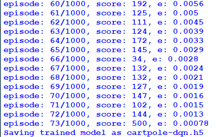
self.replay()For me, the model reached a 500 score in the 73rd step; here, my model was saved:
DQN CartPole testing part
So now, when you have trained your model, it's time to test it! Comment agent.run() line and uncomment agent.test(). And check how your first DQN model works!
if __name__ == "__main__":
    agent = DQNAgent()
    #agent.run()
    agent.test()
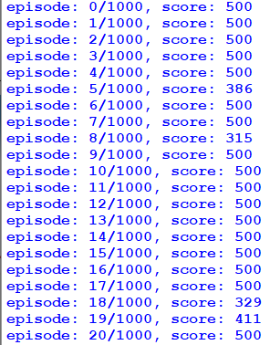
So here are 20 test episodes of our trained model. As you can see, 16 times it hit the maximum score, it would be interesting what is the maximum score it could beat, but sadly limit is 500:
And here is a short gif, which shows how our agent performs:
Conclusion:
We reached our goal for this task. A short recap of what we did:
- Learned how DQN works;
- Wrote simple DQN model;
- Taught NN model to play CartPole game.
This is the end of this tutorial. I challenge you to try creating your own RL agents! Let me know how they perform in solving the cartpole problem. Furthermore, stay tuned for more future tutorials.