LunarLander-v2 with Proximal Policy Optimization

Welcome to another part of my step-by-step reinforcement learning tutorial with gym and TensorFlow 2. I'll show you how to implement a Reinforcement Learning algorithm known as Proximal Policy Optimization (PPO) for teaching an AI agent how to land a rocket (Lunarlander-v2). By the end of this tutorial, you'll get an idea of how to apply an on-policy learning method in an actor-critic framework to learn navigating any discrete game environment. Next, followed by this tutorial I will create a similar tutorial with a continuous environment. I'll show you what these terms mean in the context of the PPO algorithm, and also I'll implement them in Python with the help of TensorFlow 2.

First, you should start with installing our game environment: pip install gym[all], pip install box2d-py. If you face some problems with installation, you can find detailed instructions on the openAI/gym GitHub page.

Note: The code for this and my entire reinforcement learning tutorial series is available in the following link: GitHub.

I'm using the openAI gym environment for this tutorial, but you can use any game environment, make sure it supports OpenAI's Gym API in Python. If you want to adapt code for other environments, make sure your inputs and outputs are correct.

If you cloned my GitHub repository, install the system dependencies and python packages required for this project. Make sure you select the correct CPU/GPU version of TensorFlow appropriate for your system: pip install -r ./requirements.txt

Running the LunarLander-v2 Environment

Now that we have the game installed let's try to test whether it runs correctly on your system or not.

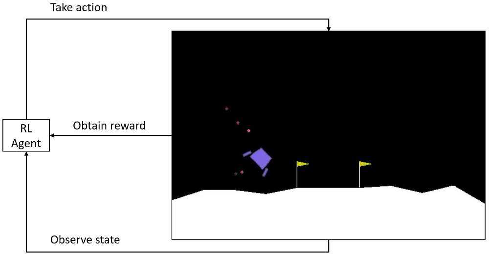
A typical Reinforcement Learning setup works by having an AI agent interact with our environment. The agent observes the current state of our environment and, based on some policy, decides to take a particular action. This action is then relayed back to the environment, which moves forward by one step. This generates a reward that indicates whether the action taken was positive or negative in the context of the game being played. Using this reward as feedback, the agent tries to figure out how to modify its existing policy to obtain better rewards in the future.

Quoted details about LunarLander-v2 (discrete environment):

Landing pad is always at coordinates (0,0). Coordinates are the first two numbers in state vector. Reward for moving from the top of the screen to landing pad and zero speed is about 100..140 points. If lander moves away from landing pad it loses reward back. Episode finishes if the lander crashes or comes to rest, receiving additional -100 or +100 points. Each leg ground contact is +10. Firing main engine is -0.3 points each frame. Solved is 200 points. Landing outside landing pad is possible. Fuel is infinite, so an agent can learn to fly and then land on its first attempt. Four discrete actions available: do nothing, fire left orientation engine, fire main engine, fire right orientation engine.

This quote provides enough details about the action and state space. Also, I observed that there is some random wind in the environment that influences the Ship's direction.

Action space (Discrete): 0-Do nothing, 1-Fire left engine, 2-Fire down the engine, 3-Fire right engine.

So now, let's go ahead and implement this for a random-action AI agent interacting with this environment. Create a new python file named random_agent.py and execute the following code:

import gym
import random

env = gym.make("LunarLander-v2")

def Random_games():
    # Each of this episode is its own game.
    for episode in range(10):
        env.reset()
        # this is each frame, up to 500...but we wont make it that far with random.
        while True:
            # This will display the environment
            # Only display if you really want to see it.
            # Takes much longer to display it.
            env.render()
            
            # This will just create a sample action in any environment.
            # In this environment, the action can be any of one how in list on 4, for example [0 1 0 0]
            action = env.action_space.sample()

            # this executes the environment with an action, 
            # and returns the observation of the environment, 
            # the reward, if the env is over, and other info.
            next_state, reward, done, info = env.step(action)
            
            # lets print everything in one line:
            print(next_state, reward, done, info, action)
            if done:
                break
                
Random_games()

This creates an environment object env for the LunarLander-v2 gym scenario where our player spawns at the top of the screen and has to score an empty goal on the right side. If you see a Spaceship on your screen taking random actions in the game, congratulations, everything is set up correctly, and we can start implementing the PPO algorithm!

Proximal Policy Optimization (PPO)

The PPO algorithm was introduced by the OpenAI team in 2017 and quickly became one of the most popular Reinforcement Learning methods that pushed all other RL methods at that moment aside. PPO involves collecting a small batch of experiences interacting with the environment and using that batch to update its decision-making policy. Once the policy is updated with that batch, the experiences are thrown away, and a newer batch is collected with the newly revised policy. This is why it is an "on-policy learning" approach where the experience samples collected are only helpful for updating the current policy.

The main idea is that the new policy should not be too far from the old policy after an update. For that, PPO uses clipping to avoid too large updates. This leads to minor variance in training at the cost of some bias but ensures smoother training and makes sure the agent does not go down to an unrecoverable path of taking senseless actions. So, let's go ahead and break down our agent into more details and see how it defines and updates its policy.

The Actor-Critic model's structure

PPO uses the Actor-Critic approach for the agent. This means that it uses two models, one called the Actor and the other called Critic:

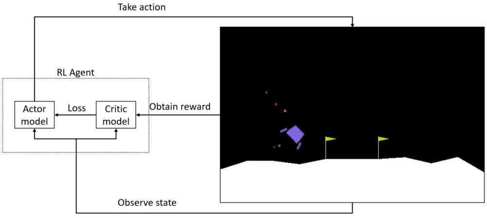
The Actor model

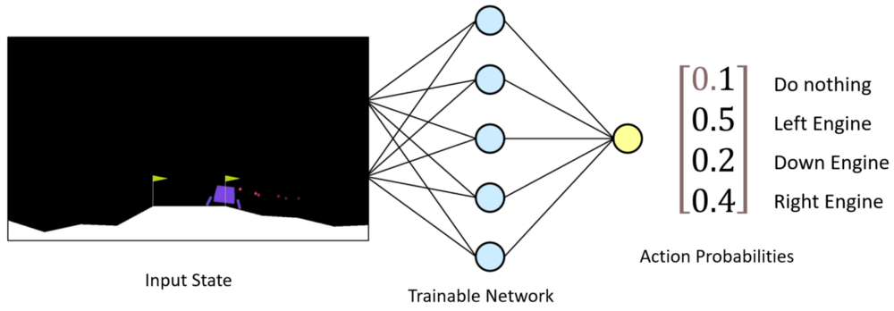
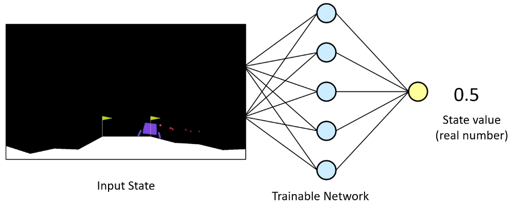
The Actor model performs the task of learning what action to take under a particular observed state of the environment. In LunarLander-v2 case, it takes eight values list of the game as input which represents the current state of our rocket and gives a particular action what engine to fire as output:

So, let's implement this by creating an Actor class:

class Actor_Model:
    def __init__(self, input_shape, action_space, lr, optimizer):
        X_input = Input(input_shape)
        self.action_space = action_space

        X = Dense(512, activation="relu", kernel_initializer=tf.random_normal_initializer(stddev=0.01))(X_input)
        X = Dense(256, activation="relu", kernel_initializer=tf.random_normal_initializer(stddev=0.01))(X)
        X = Dense(64, activation="relu", kernel_initializer=tf.random_normal_initializer(stddev=0.01))(X)
        output = Dense(self.action_space, activation="softmax")(X)

        self.Actor = Model(inputs = X_input, outputs = output)
        self.Actor.compile(loss=self.ppo_loss, optimizer=optimizer(lr=lr))

    def ppo_loss(self, y_true, y_pred):
        # Defined in https://arxiv.org/abs/1707.06347
        advantages, prediction_picks, actions = y_true[:, :1], y_true[:, 1:1+self.action_space], y_true[:, 1+self.action_space:]
        LOSS_CLIPPING = 0.2
        ENTROPY_LOSS = 0.001
        
        prob = actions * y_pred
        old_prob = actions * prediction_picks

        prob = K.clip(prob, 1e-10, 1.0)
        old_prob = K.clip(old_prob, 1e-10, 1.0)

        ratio = K.exp(K.log(prob) - K.log(old_prob))
        
        p1 = ratio * advantages
        p2 = K.clip(ratio, min_value=1 - LOSS_CLIPPING, max_value=1 + LOSS_CLIPPING) * advantages

        actor_loss = -K.mean(K.minimum(p1, p2))

        entropy = -(y_pred * K.log(y_pred + 1e-10))
        entropy = ENTROPY_LOSS * K.mean(entropy)
        
        total_loss = actor_loss - entropy

        return total_loss

    def predict(self, state):
        return self.Actor.predict(state)

Here, we first define the input shape input_shape for our neural net, which is our environment action_space. action_space is the total number of possible actions available in the current environment and will be the total number of output nodes of the neural net. I am using three deep superficial layers of Neural Network with the following neurons [512, 256, 64]. The last layer is the classification layer, with the softmax activation function added on top of this trainable feature extractor layer. This way, our agent will learn to predict the correct actions. Everything is combined and compiled with a custom PPO loss function.

Custom PPO loss

This is the most crucial part of the Proximal Policy Optimization algorithm. So let's first understand this loss function.

Probabilities (prob) and old probabilities (old_prob) of actions indicate the policy that our Actor Neural Network model defines. By training this model, we want to improve these probabilities to give us better and better actions over time. A significant problem in some Reinforcement Learning approaches is that once our model adopts a bad policy, it only takes terrible actions in the game. Hence, we cannot generate any good actions from there on, leading us down an unrecoverable path in training. PPO tries to address this by only making minor updates to the model in an update step, thereby stabilizing the training process.

The above PPO loss code can be explained as follows:

• PPO uses a ratio between the newly updated policy and the old policy in the update step. Computationally, it is easier to represent this in the log form: ratio = K.exp(K.log(prob) — K.log(old_prob));
• Using this ratio, we can decide how much of a policy change we are willing to tolerate. Hence, we use a clipping parameter LOSS_CLIPPING to ensure we only make the maximum percent change to our policy at a time. Paper suggests using this value as 0.2:
  p1=ratio*advantages
p2=K.clip(ratio,min_value=1 — LOSS_CLIPPING, max_value=1+LOSS_CLIPPING)*advantages;
• Actor loss is calculating by simply getting a negative mean of element-wise minimum value of p1 and p2;
• Adding an entropy term is optional, but it encourages our actor model to explore different policies. An entropy beta parameter can control the degree to which we want to experiment.

The Critic model

We send the action predicted by the Actor to our environment and observe what happens in the game. If something positive happens due to our action, like landing a spaceship, then the environment sends back a positive response in the form of a reward. But if our spaceship falls, we receive a negative reward. These rewards are taken in by training our Critic model:

The primary role of the Critic model is to learn to evaluate if the action taken by the Actor led our environment to be in a better state or not and give its feedback to the Actor. Critic outputs an actual number indicating a rating (Q-value) of the action taken in the previous state. By comparing this rating obtained from the Critic, the Actor can compare its current policy with a new policy and decide how it wants to improve itself to take better actions.

Same as with Actor, we implement the Critic:

class Critic_Model:
    def __init__(self, input_shape, action_space, lr, optimizer):
        X_input = Input(input_shape)
        old_values = Input(shape=(1,))

        V = Dense(512, activation="relu", kernel_initializer='he_uniform')(X_input)
        V = Dense(256, activation="relu", kernel_initializer='he_uniform')(V)
        V = Dense(64, activation="relu", kernel_initializer='he_uniform')(V)
        value = Dense(1, activation=None)(V)

        self.Critic = Model(inputs=[X_input, old_values], outputs = value)
        self.Critic.compile(loss=[self.critic_PPO2_loss(old_values)], optimizer=optimizer(lr=lr))

    def critic_PPO2_loss(self, values):
        def loss(y_true, y_pred):
            LOSS_CLIPPING = 0.2
            clipped_value_loss = values + K.clip(y_pred - values, -LOSS_CLIPPING, LOSS_CLIPPING)
            v_loss1 = (y_true - clipped_value_loss) ** 2
            v_loss2 = (y_true - y_pred) ** 2
            
            value_loss = 0.5 * K.mean(K.maximum(v_loss1, v_loss2))
            #value_loss = K.mean((y_true - y_pred) ** 2) # standard PPO loss
            return value_loss
        return loss

    def predict(self, state):
        return self.Critic.predict([state, np.zeros((state.shape[0], 1))])

As you can see, the structure of the Critic neural net is almost the same as the Actor (but you can change it, test what structure is best for you). The only major difference being, the final layer of Critic outputs an actual number. Hence, the activation used is None (we can use tanh also) and not softmax since we do not need a probability distribution here like the Actor. Same as in Actor, I use the custom PPO2 critic function, where clipping is used to avoid too large updates. I can't give you a brief explanation about this custom function because I couldn't find the paper where it would be explained.

An essential step in the PPO algorithm is to run through this entire loop with the two models for a fixed number of steps known as PPO steps. So essentially, we are interacting with our environment for a certain number of steps and collecting the states, actions, rewards, etc., which we will use for training. Still, before training, we need to process our rewards that our model can learn from it.

Generalized Advantage Estimation (GAE)

Advantage - can be defined as measuring how much better off we can be by taking a particular action when we are in a specific state. We want to use the rewards that we collected at each time step and calculate how much of an advantage we could obtain by taking the action that we took. So if we took a good move, we want to calculate how much better off we were by taking that action. We want to do that in the short run and over a more extended period. This way, even if we do not immediately score a goal in the next step, we still look at a few steps after that action into the longer future to see if we received a better reward.

If you were in reinforcement learning for a while, you probably faced a discounted episode reward strategy; that's one of the most straightforward and most used strategies to process rewards. But there is a known method called Generalized Advantage Estimation (GAE) which I'll use to get better results.

This is the GAE algorithm implemented in our code as follows:

def get_gaes(self, rewards, dones, values, next_values, gamma = 0.99, lamda = 0.9, normalize=True):
    deltas = [r + gamma * (1 - d) * nv - v for r, d, nv, v in zip(rewards, dones, next_values, values)]
    deltas = np.stack(deltas)
    gaes = copy.deepcopy(deltas)
    for t in reversed(range(len(deltas) - 1)):
        gaes[t] = gaes[t] + (1 - dones[t]) * gamma * lamda * gaes[t + 1]

    target = gaes + values
    if normalize:
        gaes = (gaes - gaes.mean()) / (gaes.std() + 1e-8)
    return np.vstack(gaes), np.vstack(target)

Let's take a look at how this algorithm works using the batch of experiences we have collected (rewards, dones, values, next_values):

• Here, a dones is used because if the game is over, we are not interested in what our next value will be, we use our last received reward without discount;
• Gamma is nothing but a constant known as a discount factor to reduce the value of the future state since we want to emphasize more on the current state than a future state. We can consider this as getting a reward earlier is more valuable than rewarding in the future. Hence we discount future rewards so that we can put more value to present good action;
• Lambda is a smoothing parameter used for reducing the variance in training which makes it more stable. This gives us the advantage of taking action both in the short and long term;
• In the last step, we are simply normalizing the result and divide it by standard deviation.

It's hard to understand everything in the minor details, and I am not sure if I understand it correctly. So if you want to get details of it, I recommend reading the paper.

Model Training

Now we can finally start the model training. For this, I use mostly known the fit function of Keras in the following code:

def replay(self, states, actions, rewards, predictions, dones, next_states):
    # reshape memory to appropriate shape for training
    states = np.vstack(states)
    next_states = np.vstack(next_states)
    actions = np.vstack(actions)
    predictions = np.vstack(predictions)

    # Get Critic network predictions 
    values = self.Critic.predict(states)
    next_values = self.Critic.predict(next_states)

    # Compute discounted rewards and advantages
    advantages, target = self.get_gaes(rewards, dones, np.squeeze(values), np.squeeze(next_values))

    # stack everything to numpy array
    # pack all advantages, predictions and actions to y_true and when they are received
    # in custom PPO loss function we unpack it
    y_true = np.hstack([advantages, predictions, actions])
    
    # training Actor and Critic networks
    a_loss = self.Actor.Actor.fit(states, y_true, epochs=self.epochs, verbose=0, shuffle=self.shuffle)
    c_loss = self.Critic.Critic.fit([states, values], target, epochs=self.epochs, verbose=0, shuffle=self.shuffle)

You should now see on your screen the model taking different actions and collecting rewards from the environment. At the beginning of the training process, the actions may seem random as the randomly initialized model explores the game environment.

For the first seven episodes I extracted rewards and advantages that we use to train our model; these are the scores of our first episodes:

episode: 1/10000, score: -417.70159222820666, average: -417.70
episode: 2/10000, score: -117.885796622671, average: -267.79
episode: 3/10000, score: -178.31907523778347, average: -237.97
episode: 4/10000, score: -290.7847529889836, average: -251.17
episode: 5/10000, score: -184.27964347631453, average: -237.79
episode: 6/10000, score: -84.42238335425903, average: -212.23
episode: 7/10000, score: -107.02611401430872, average: -197.20

And these are the rewards(orange) and advantage(blue) curves:

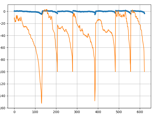
You might see that when our agent loses, advantages drop significantly also.

Tying it all together

Now that our actors and critic models have defined covered reward and training parts, we can use them to interact with the gym environment for a fixed number of steps and collect our experiences. These experiences will be used to update the policies of our models after we have a specific batch of such samples. This is how to implement the loop collecting such sample experiences:

def run_batch(self): # train every self.Training_batch episodes
    state = self.env.reset()
    state = np.reshape(state, [1, self.state_size[0]])
    done, score, SAVING = False, 0, ''
    while True:
        # Instantiate or reset games memory
        states, next_states, actions, rewards, predictions, dones = [], [], [], [], [], []
        for t in range(self.Training_batch):
            self.env.render()
            # Actor picks an action
            action, action_onehot, prediction = self.act(state)
            # Retrieve new state, reward, and whether the state is terminal
            next_state, reward, done, _ = self.env.step(action)
            # Memorize (state, action, reward) for training
            states.append(state)
            next_states.append(np.reshape(next_state, [1, self.state_size[0]]))
            actions.append(action_onehot)
            rewards.append(reward)
            dones.append(done)
            predictions.append(prediction)
            # Update current state
            state = np.reshape(next_state, [1, self.state_size[0]])
            score += reward
            if done:
                self.episode += 1
                average, SAVING = self.PlotModel(score, self.episode)
                print("episode: {}/{}, score: {}, average: {:.2f} {}".format(self.episode, self.EPISODES, score, average, SAVING))

                state, done, score, SAVING = self.env.reset(), False, 0, ''
                state = np.reshape(state, [1, self.state_size[0]])
                
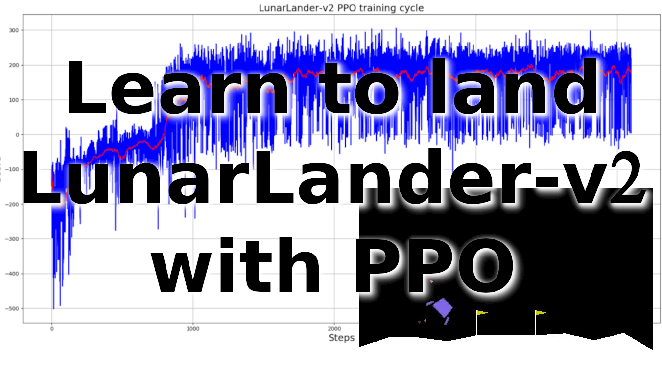
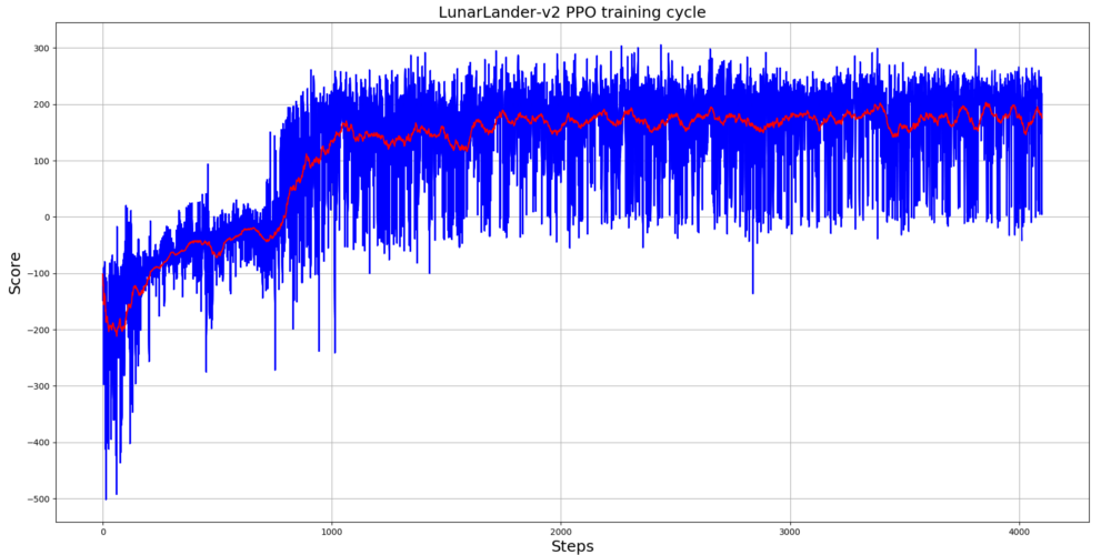
        self.replay(states, actions, rewards, predictions, dones, next_states)

I trained LunarLander-v2 agent for 4k+ steps, and from bellow graph, you can see that it took only 1k steps to start getting maximum rewards; this is amazing results:

Conclusion:

I hope this tutorial will give you a good idea of the most popular PPO algorithm. I tried to write my code as simple and understandable that every one of you could move on and implement whatever discrete environment you wanted. Also, I implemented multiprocessing training (everything is on GitHub) to execute multiple environments in parallel to collect more training samples and solve more complicated games.

That's all for this tutorial; in the next part, I'll implement continuous PPO loss to solve more challenging games like BipedalWalker-v3. Stay tuned!

Resources:

[1.] Schulman, J., Wolski, F., Dhariwal, P., Radford, A. and Klimov, O., 2017. Proximal policy optimization algorithms. arXiv preprint arXiv:1707.06347.
[2.] Schulman, J., Moritz, P., Levine, S., Jordan, M. and Abbeel, P., 2015. High-dimensional continuous control using generalized advantage estimation. arXiv preprint arXiv:1506.02438.